Neural Networks

1. Model Representation I

Let’s examine how we will represent a hypothesis function using neural networks. At a very simple level, neurons are basically computational units that take inputs (dendrites) as electrical inputs (called “spikes”) that are channeled to outputs (axons). In our model, our dendrites are like the input features $x_1\cdots x_n$ , and the output is the result of our hypothesis function. In this model our $x_0$ input node is sometimes called the “bias unit.” It is always equal to 1. In neural networks, we use the same logistic function as in classification, $\frac{1}{1+e^{-{\theta }^{T}x}}$ , yet we sometimes call it a sigmoid (logistic) activation function. In this situation, our “theta” parameters are sometimes called “weights”.

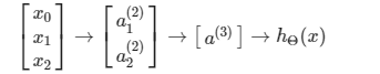
Our input nodes (layer 1), also known as the “input layer”, go into another node (layer 2), which finally outputs the hypothesis function, known as the “output layer”.

We can have intermediate layers of nodes between the input and output layers called the “hidden layers.”

This is saying that we compute our activation nodes by using a 3×4 matrix of parameters. We apply each row of the parameters to our inputs to obtain the value for one activation node. Our hypothesis output is the logistic function applied to the sum of the values of our activation nodes, which have been multiplied by yet another parameter matrix ${\Theta }^{(2)}$ containing the weights for our second layer of nodes.

---

让我们检查一下如何使用神经网络来表示一个假设函数。最简单的情况下，神经元基本上是计算单位，将输入(树突)作为电输入(称为“尖峰”)，然后传导到输出(轴突)。 在我们的模型中，我们的树突就像输入特征 $x_1\cdots x_n$，而输出则是我们的假设函数的结果。 在这个模型中，我们的 $x_0$ 输入节点有时被称为“偏差单位”，它总是等于1。 在神经网络中，我们使用与分类相同的logistic函数 $\frac{1}{1+e^{-{\theta }^{T}x}}$ ，但我们有时称其为sigmoid (logistic)激活函数。 在这种情况下，我们的“θ”参数有时被称为“权值”。

我们的输入节点(layer 1)，也称为“输入层”，进入另一个节点(layer 2)，最后输出假设函数，称为“输出层”。

我们可以在输入和输出层之间有称为“隐藏层”的中间节点层。


这就是说，我们通过使用3×4参数矩阵来计算激活节点。 我们将每一行参数应用于输入，以获得一个激活节点的值。 含有第二层参数结点值的矩阵 ${\theta }^{(2)}$ 乘以激活节点 a⁽²⁾ 作为 logistic 函数的输入值，得到的结果为假设输出。

2. Model Representation II

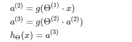
In this section we’ll do a vectorized implementation of the above functions. We’re going to define a new variable $z_k^{(j)}$ that encompasses the parameters inside our g function. In our previous example if we replaced by the variable z for all the parameters we would get：
$$\begin{gathered} a_1^{(2)}=g(z_1^{(2)}) \\ {a}_2^{(2)}=g(z_2^{(2)}) \\ {a}_3^{(2)}=g(z_3^{(2)}) \end{gathered}$$
In other words, for layer j=2 and node k, the variable z will be:
$z_k^{(2)}={\Theta }_{k,0}^{(1)}{x}_0+{\Theta }_{k,1}^{(1)}{x}_1+{\Theta }_{k,n}^{(1)}{x}_n$

The vector representation of x and $z^j$ is:
$$x=\left[\begin{array}{c}{x}_0\\ x_1\\ \cdots \\ x_n\end{array}\right]z^{(j)}=\left[\begin{array}{c}{z}_1^j\\ z_2^j\\ \cdots \\ z_n^j\end{array}\right]$$

Setting $x=a^{(1)}$ , we can rewrite the equation as:
$z^{(j)}={\Theta }^{(j-1)}{a}^{(j-1)}$

We are multiplying our matrix ${\Theta }^{(j-1)}$ with dimensions $s_j\times (n+1)$ (where $s_j$ is the number of our activation nodes) by our vector $a^{(j-1)}$ with height (n+1). This gives us our vector $z^{(j)}$z with height $s_j$ . Now we can get a vector of our activation nodes for layer j as follows:
$a^{(j)}=g(z(j))$

Where our function g can be applied element-wise to our vector $z^{(j)}$ .

We can then add a bias unit (equal to 1) to layer j after we have computed $a^{(j)}$. This will be element $a_0^{(j)}$ and will be equal to 1. To compute our final hypothesis, let’s first compute another z vector:
$z^{(j+1)}={\Theta }^{(j)}{a}^{(j)}$

We get this final z vector by multiplying the next theta matrix after ${\Theta }^{(j-1)}$ with the values of all the activation nodes we just got. This last theta matrix ${\Theta }^{(j)}$ will have only one row which is multiplied by one column $a^{(j)}$ so that our result is a single number. We then get our final result with:
$h_{\Theta }(x)=a^{(j+1)}=g(z^{(j+1)})$

---

在本节中，我们将对上述函数进行矢量化实现。 我们将定义一个新变量$z_k^{(j)}$，它是g函数中的参数。 在我们之前的例子中，如果我们用变量z替换所有的参数，我们将得到:
$$\begin{gathered} a_1^{(2)}=g(z_1^{(2)}) \\ {a}_2^{(2)}=g(z_2^{(2)}) \\ {a}_3^{(2)}=g(z_3^{(2)}) \end{gathered}$$
换句话说，对于层 j = 2中的节点k，变量z为:
$z_k^{(2)}={\Theta }_{k,0}^{(1)}{x}_0+{\Theta }_{k,1}^{(1)}{x}_1+{\Theta }_{k,n}^{(1)}{x}_n$

x和$z^j$的向量表示为:
$$x=\left[\begin{array}{c}{x}_0\\ x_1\\ \cdots \\ x_n\end{array}\right]z^{(j)}=\left[\begin{array}{c}{z}_1^j\\ z_2^j\\ \cdots \\ z_n^j\end{array}\right]$$

设$x=a^{(1)}$，可以将方程改写为:
$z^{(j)}={\Theta }^{(j-1)}{a}^{(j-1)}$

我们用维数为 $s_j\times (n+1)$ 的矩阵${\theta }^{(j-1)}$（其中$s_j$是激活节点的数目）乘以高度为（n+1）的向量$a^{(j-1)}$。 这就得到了高度为 $s_j$ 的向量$z^{(j)}$。 现在我们可以得到第j层的激活节点的向量，如下所示:
$a^{(j)}=g(z^{(j)})$

我们的函数g可以被应用到向量$z^{(j)}$上。

然后，在我们计算了$a^{(j)}$之后，我们可以在第j层添加一个偏差单位(等于1)。 这是元素$a_0^{(j)}$，它等于1。 为了计算最终的假设，我们先计算另一个z向量:
$z^{(j+1)}={\Theta }^{(j)}{a}^{(j)}$

我们通过将 ${\theta }^{(j-1)}$ 后面的下一个矩阵与我们刚刚得到的所有激活节点的值相乘，得到最后的z向量。 这个最后的矩阵${\theta }^{(j)}$将只有一行乘以一列$a^{(j)}$，因此我们的结果是一个单一的数字。 然后我们得到我们的最终结果:
$h_{}(x)=a^{(j+1)}=g(z^{(j+1)})$

3. Examples and Intutions I

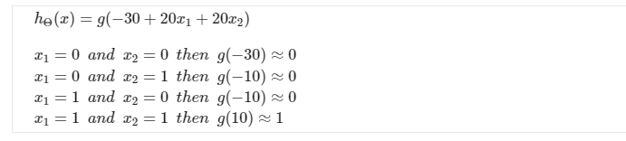
A simple example of applying neural networks is by predicting $x_1$ AND $x_2$, which is the logical ‘and’ operator and is only true if both $x_1$ and $x_2$ are 1.

This will cause the output of our hypothesis to only be positive if both $x_1$ and $x_2$ are 1.

So we have constructed one of the fundamental operations in computers by using a small neural network rather than using an actual AND gate. Neural networks can also be used to simulate all the other logical gates. The following is an example of the logical operator ‘OR’, meaning either $x_1$ is true of $x_2$ is true, or both:

---

一个简单的应用神经网络的例子是通过预测$x_1$和$x_2$，这是逻辑的’ AND '算子，只有当$x_1$和$x_2$都是1时才成立。

这将导致我们的假设的输出只有当$x_1$和$x_2$都是1时才为正。

所以我们用一个小的神经网络而不是实际的“AND”门构建了计算机的一个基本操作。 神经网络也可以用来模拟所有其他逻辑门。 下面是逻辑运算符’OR’的例子，表示$x_1$为真或$x_2$为真，或两者都为真:

4. Examples and Intutions II

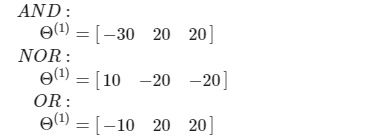
The ${\Theta }^{(1)}$matrices for AND, NOR, and OR are:

We can combine these to get the XNOR logical operator (which gives 1 if $x_1$ and $x_2$ are both 0 or both 1).

---

AND, NOR和OR的${\Theta }^{(1)}$矩阵为:

我们可以将它们组合起来得到XNOR逻辑运算符(如果$x_1$和$x_2$都是0或都是1，则得到1)。

5. Multiclass Classification

To classify data into multiple classes, we let our hypothesis function return a vector of values. Say we wanted to classify our data into one of four categories. We will use the following example to see how this classification is done. This algorithm takes as input an image and classifies it accordingly:

We can define our set of resulting classes as y:

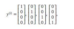
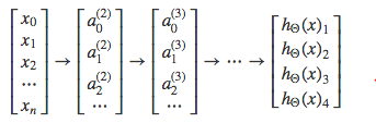
Each $y^{(i)}$ represents a different image corresponding to either a car, pedestrian, truck, or motorcycle. The inner layers, each provide us with some new information which leads to our final hypothesis function. The setup looks like:

---

为了将数据分类为多个类，我们让假设函数返回一个向量。 假设我们想将数据分为四类。 我们将使用下面的示例来了解如何进行这种分类。 该算法以一幅图像作为输入，并对其进行分类:

我们可以将结果类集定义为y:

每个$y^{(i)}$代表一个不同的图像，分别对应于汽车、行人、卡车或摩托车。 内层中，每一层都为我们提供了一些新的信息这些信息会引导我们最终的假设函数。 设置如下:

Exercise 3：多分类任务和神经网络

【吴恩达机器学习】Week4 编程作业ex3——多分类任务和神经网络

全部作业代码

MLExercise_Ng