引言

上一节介绍了卡尔曼滤波以及其在滤波问题中的求解思想，本节将介绍粒子滤波(Particle Filter)，并针对重要性采样的缺陷介绍序列重要性采样(Sequential Importance Sampling)。

回顾：动态模型

动态模型的划分

在隐马尔可夫模型(Hidden Markov Model,HMM)与卡尔曼滤波介绍(Karlman Filter)中介绍了动态模型(Dynamic Model)的概念。其概率图模型表示如下：

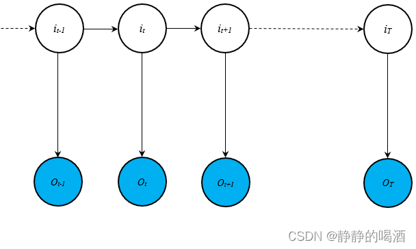
在关于变量概率的求解过程中，包含动态模型的两个假设：

• 齐次马尔可夫假设：该假设是由马尔可夫链(Markov Chain)中延伸过来的假设。文字描述为：给定当前状态变量$i_t$的条件下，未来的状态变量只与当前状态相关，与过去状态无关。对应数学符号表示如下：
  这里以‘一阶齐次马尔可夫假设’为例。
  $$\mathcal{P}(i_{t+1}\mid i_1,i_2,\cdots ,i_t)=\mathcal{P}(i_{t+1}\mid i_t)$$
• 观测独立性假设：某时刻观测变量$o_t$的后验概率，只与对应时刻的隐变量$i_t$相关，与其他时刻的任意变量无关。对应数学符号表示如下：
  需要注意的点:所有‘动态模型’均服从该假设，而不仅仅是‘隐马尔可夫模型’。
  $$\mathcal{P}(o_t\mid i_1,\cdots ,i_T,o_1,\cdots ,o_T)=\mathcal{P}(o_t\mid i_t)$$

从隐变量$i_t(i=1,2,\cdots ,T)$的基本类型角度进行划分，可划分为如下形式：

• 隐变量是离散型随机变量的隐马尔可夫模型：隐马尔可夫模型对观测变量的基本类型没有过多要求。可以是连续，也可以是离散；
  为计算方便起见，假设观测变量也服从离散型随机变量，因而隐马尔可夫模型的模型参数 表示如下：
  $$\lambda =(\pi ,\mathcal{A},\mathcal{B})$$
  其中$\pi$表示初始时刻隐变量的概率结果$\mathcal{P}(i_1)$。由于是离散型随机变量，可以将概率分布表示为如下形式：

  离散结果	$q_1$	$q_2$	$\cdots$	$q_{\mathcal{K}}$
  对应概率	$\mathcal{P}(i_1=q_1)$	$\mathcal{P}(i_1=q_2)$	$\cdots$	$\mathcal{P}(i_1=q_{\mathcal{K}})$

  $\mathcal{A}$为状态转移矩阵，矩阵中的每个元素表示相邻时刻隐变量的条件概率结果：
  $$a_{ij}=\mathcal{P}(i_t=q_j\mid i_{t-1}=q_i)$$
  $\mathcal{B}$为发射矩阵，矩阵中的每个元素表示某时刻隐变量与对应时刻观测变量之间的条件概率结果：
  $$b_j(k)=\mathcal{P}(o_t=v_k\mid i_t=q_j)$$

• 隐变量是连续型随机变量的有卡尔曼滤波、粒子滤波。其中卡尔曼滤波的模型参数 表示如下：
  $$\lambda =(\mathcal{A},\mathcal{B},\mathcal{C},\mathcal{D},\mathcal{Q},\mathcal{R},{\mu }_1,{\Sigma }_1)$$

  并且卡尔曼滤波要求相邻隐变量之间、隐变量与对应观测变量之间属于线性关系。并且噪声服从高斯分布：
  $$\begin{array}{rl}\mathcal{P}(i_t\mid i_{t-1})& \sim \mathcal{N}(\mathcal{A}\cdot i_{t-1}+\mathcal{B},\mathcal{Q})\\ \mathcal{P}(o_t\mid i_t)& \sim \mathcal{N}(\mathcal{C}\cdot i_t+\mathcal{D},\mathcal{R})\end{array}$$
  并且卡尔曼滤波中初始时刻隐变量的概率分布$\mathcal{P}(i_1)$服从高斯分布：
  $$\mathcal{P}(i_1)\sim \mathcal{N}({\mu }_1,{\Sigma }_1)$$

动态模型处理的任务

在动态模型基本介绍中已经提到了动态模型的相关处理任务。这里不再赘述。不同模型对于任务处理的侧重点 有所不同：

• 隐马尔可夫模型更关注 求值问题(Evaluation)与学习任务(Learning)：
  $$\begin{array}{r}\mathcal{P}(\mathcal{O}\mid \lambda )=\mathcal{P}(o_1,o_2,\cdots ,o_T\mid \lambda )\\ \hat{\lambda }=\underset{\lambda }{\mathrm{argmax}}\mathcal{P}(\mathcal{O}\mid \lambda )\lambda =(\pi ,\mathcal{A},\mathcal{B})\end{array}$$
• 卡尔曼滤波、粒子滤波更关注 滤波问题(Filtering)：
  $$\mathcal{P}(i_t\mid o_1,\cdots ,o_t)$$
  而卡尔曼滤波处理滤波问题使用先预测，再对预测修正的迭代过程：
  • 预测步骤(Prediction)：
    $$\begin{array}{rl}\mathcal{P}(i_t\mid o_1,\cdots ,o_{t-1})& ={\int }_{i_{t-1}}\mathcal{P}(i_t\mid i_{t-1})\cdot \mathcal{P}(i_{t-1}\mid o_1,\cdots ,o_{t-1})d{i}_{t-1}\end{array}$$
  • 更新步骤(Update)：
    $$\begin{array}{rl}\mathcal{P}(i_t\mid o_1,\cdots ,o_t)& =\frac{\mathcal{P}(o_1,\cdots ,o_{t-1})}{\mathcal{P}(o_{,}\cdots ,o_t)}\cdot \left[\mathcal{P}(o_t\mid i_t)\cdot \mathcal{P}(i_t\mid o_1,\cdots ,o_{t-1})\right]\\ & \propto \mathcal{P}(o_t\mid i_t)\cdot \mathcal{P}(i_t\mid o_1,\cdots ,o_{t-1})\end{array}$$

粒子滤波关于滤波问题的求解

粒子滤波在动态模型中最显著的特点是：相邻时刻隐变量之间、观测变量与对应时刻隐变量之间的关联关系均是非线性的，并且对应噪声也是非高斯分布的。

由于卡尔曼滤波中变量之间的优质特性，因此可以通过高斯分布的一系列变换在每一次预测步骤(Prediction)与更新步骤(Update)中能够精确得到隐变量$i_t$概率的精确结果。

而粒子滤波对于变量之间的关联关系是模糊的，从而没有办法得到解析解。因此，需要借助采样(Sampling)的方式得到隐变量$i_t$概率的近似结果。

蒙特卡洛方法

蒙特卡洛方法本身是近似推断(Approximate Inference)中的一系列方法。

推断(Inference)在概率图模型(六)推断基本介绍中提到，其本质上是求解变量的概率。在包含隐变量$\mathcal{Z}$的任务中，推断的目标是求解给定观测变量$\mathcal{X}$的条件下，隐变量$\mathcal{Z}$的后验概率结果$\mathcal{P}(\mathcal{Z}\mid \mathcal{X})$。

由于分布的复杂性，$\mathcal{P}(\mathcal{Z}\mid \mathcal{X})$可能无法直接求解，并且$\mathcal{P}(\mathcal{Z}\mid \mathcal{X})$在应用过程中，我们更加关心的是$\mathcal{P}(\mathcal{Z}\mid \mathcal{X})$分布下的期望结果：
$${\mathbb{E}}_{\mathcal{Z}\mid \mathcal{X}}[f(\mathcal{X})]={\int }_{\mathcal{Z}}f(\mathcal{X})\cdot \mathcal{P}(\mathcal{Z}\mid \mathcal{X})d\mathcal{Z}$$
而蒙特卡洛方法(Monte Carlo Method)通过采样的方式直接近似求解${\mathbb{E}}_{\mathcal{Z}\mid \mathcal{X}}[f(\mathcal{X})]$：

• 从$\mathcal{P}(\mathcal{Z}\mid \mathcal{X})$分布中采集$N$个样本：
  虽然$\mathcal{P}(\mathcal{Z}\mid \mathcal{X})$的概率分布我们不能精确得知，但并不影响采集样本。
  $$z^{(1)},z^{(2)},\cdots ,z^{(N)}\sim \mathcal{P}(\mathcal{Z}\mid \mathcal{X})$$
• 根据大数定律，通过样本均值的形式求解${\mathbb{E}}_{\mathcal{Z}\mid \mathcal{X}}[f(\mathcal{X})]$：
  $${\mathbb{E}}_{\mathcal{Z}\mid \mathcal{X}}[f(\mathcal{X})]\approx \frac{1}{N}\sum _{i=1}^{N}f(z^{(i)})$$

重要性采样

针对$\mathcal{P}(\mathcal{Z}\mid \mathcal{X})$过于复杂，亦或是维度过高，导致 无法高效地从$\mathcal{P}(\mathcal{Z}\mid \mathcal{X})$分布中采集到样本。

通过重要性采样(Importance Sampling)方法，引入一个 简单分布/可采样的分布$\mathcal{Q}(\mathcal{Z})$并对其进行采样，通过重要性权重(Importance Weight)的筛选，从而得到有效的采样结果：
称$\mathcal{Q}(\mathcal{Z})$为‘提议分布/候选分布’。
$$\begin{array}{rl}{\mathbb{E}}_{\mathcal{Z}\mid \mathcal{X}}[f(\mathcal{X})]& ={\int }_{\mathcal{Z}}f(\mathcal{X})\cdot \mathcal{P}(\mathcal{Z}\mid \mathcal{X})d\mathcal{Z}\\ & ={\int }_{\mathcal{Z}}\mathcal{Q}(\mathcal{Z})\cdot \left[f(\mathcal{X})\cdot \frac{\mathcal{P}(\mathcal{Z}\mid \mathcal{X})}{\mathcal{Q}(\mathcal{Z})}\right]d\mathcal{Z}\\ & ={\mathbb{E}}_{\mathcal{Q}(\mathcal{Z})}\left[f(\mathcal{X})\cdot \frac{\mathcal{P}(\mathcal{Z}\mid \mathcal{X})}{\mathcal{Q}(\mathcal{Z})}\right]\end{array}$$
其中$\frac{\mathcal{P}(\mathcal{Z}\mid \mathcal{X})}{\mathcal{Q}(\mathcal{Z})}$即 重要性权重，针对上述期望形式，通过蒙特卡洛采样方法近似求解${\mathbb{E}}_{\mathcal{Z}\mid \mathcal{X}}[f(\mathcal{X})]$：
$$\begin{array}{r}{z}^{(1)},z^{(2)},\cdots ,z^{(N)}\sim \mathcal{Q}(\mathcal{Z})\\ {\mathbb{E}}_{\mathcal{Z}\mid \mathcal{X}}[f(\mathcal{X})]\approx \frac{1}{N}\sum _{i=1}^{N}f(z^{(i)})\cdot \frac{\mathcal{P}(z^{(i)})}{\mathcal{Q}(z^{(i)})}\end{array}$$

重要性采样处理滤波任务的缺陷

针对滤波问题$\mathcal{P}(i_t\mid o_1,\cdots ,o_t)$，使用重要性采样方法得到 $t$时刻第$i$次重要性采样得到的重要性权重${\mathcal{W}}_t^{(i)}$ 表示如下：
$${\mathcal{W}}_t^{(i)}=\frac{\mathcal{P}(z_t^{(i)}\mid o_1,\cdots ,o_t)}{\mathcal{Q}(z_t^{(i)}\mid o_1,\cdots ,o_t)}$$
其中，$z_t^{(i)}$表示 $t$时刻在$\mathcal{Q}(\mathcal{Z})$中采集的第$i$个样本；而需要注意的点是：观测变量$o_1,\cdots ,o_t$是给定的信息，不经过采样过程。

观察执行一次采样，需要运算的步骤(依然以$z_t^{(i)}$为例)：

• 计算$\mathcal{P}(z_t^{(i)}\mid o_1,\cdots ,o_t)$：
  $$\begin{array}{rl}\mathcal{P}(z_t^{(i)}\mid o_1,\cdots ,o_t)& =\frac{\mathcal{P}(z_t^{(i)},o_1,\cdots ,o_t)}{\mathcal{P}(o_1,\cdots ,o_t)}\\ & \propto \mathcal{P}(z_t^{(i)},o_1,\cdots ,o_t)\end{array}$$
  继续对$\mathcal{P}(z_t^{(i)},o_1,\cdots ,o_t)$进行求解。实际情况是：求解$\mathcal{P}(z_t^{(i)},o_1,\cdots ,o_t)$过于复杂，运算代价很高。

  在介绍求值问题(Evaluation)时，无论是前向算法(Forward Algorithm)还是后向算法(Backward Algorithm)，都需要从某一端开始遍历，从而时间复杂度均为$\mathcal{O}(T)$。

• 上述运算仅仅是某时刻的某一次采样结果，而整个过程一共需要采样$N\times T$次，即 每个时刻都需要采集$N$个样本，最终它的时间复杂度为$\mathcal{O}(T^2\times N)$。
  这里假设‘每一时刻采样的数量是相同的’，最终的时间复杂度只是一个粗略结果。

序列重要性采样

由于滤波问题本身是一个在线算法，一个朴素的想法是：将某时刻的重要性权重结果${\mathcal{W}}_t$与上一时刻的结果${\mathcal{W}}_{t-1}$之间建立联系，如果找到联系，可以通过迭代方式简化大量运算。

根据动态模型的性质，引入一种重要性采样的改进算法：序列重要性采样(Sequential Important Sampling,SIS)
其核心在于找出当前时刻采样的重要性权重${\mathcal{W}}_t$和上一时刻采样的重要性权重${\mathcal{W}}_{t-1}$之间的关联关系。
这里并不关注采样的编号，它只是一个采样顺序编号，没有具体用处。
$$\begin{array}{rl}{\mathcal{W}}_{t-1}& =\frac{\mathcal{P}(i_{t-1}\mid o_1,\cdots ,o_{t-1})}{\mathcal{Q}(i_{t-1}\mid o_1,\cdots ,o_{t-1})}\\ {\mathcal{W}}_t& =\frac{\mathcal{P}(i_t\mid o_1,\cdots ,o_t)}{\mathcal{Q}(i_t\mid o_1,\cdots ,o_t)}\\ {\mathcal{W}}_{t-1}& \stackrel{\text{?}}{\leftrightarrow }{\mathcal{W}}_t\end{array}$$

序列重要性采样的核心思想在于 它并没有直接求解滤波问题$\mathcal{P}(i_t\mid o_1,\cdots ,o_t)$，而是求解概率分布$\mathcal{P}(i_1,\cdots ,i_t\mid o_1,\cdots ,o_t)$

该算法的设想是：通过求解联合概率分布的比值，来近似看作滤波问题的比值。数学符号表示如下：
$${\mathcal{W}}_t=\frac{\mathcal{P}(i_t\mid o_1,\cdots ,o_t)}{\mathcal{Q}(i_t\mid o_1,\cdots ,o_t)}\propto \frac{\mathcal{P}(i_1,\cdots ,i_t\mid o_1,\cdots ,o_t)}{\mathcal{Q}(i_1,\cdots ,i_t\mid o_1,\cdots ,o_t)}$$

从下面开始，先通过个人想法来解释该设想的合理性。

对于SIS设想的个人解释

关于该式：
$${\mathcal{W}}_t=\frac{\mathcal{P}(i_t\mid o_1,\cdots ,o_t)}{\mathcal{Q}(i_t\mid o_1,\cdots ,o_t)}\propto \frac{\mathcal{P}(i_1,\cdots ,i_t\mid o_1,\cdots ,o_t)}{\mathcal{Q}(i_1,\cdots ,i_t\mid o_1,\cdots ,o_t)}$$
其中分母部分是关于$\mathcal{Q}$的分布，该分布是人为设置的简单分布，变量关系随着$\mathcal{P}$的变化而变化，因此将关注点放在$\mathcal{P}$分布中变量的关联关系上：
$$\mathcal{P}(i_t\mid o_1,\cdots ,o_t)\leftrightarrow \mathcal{P}(i_1,\cdots ,i_t\mid o_1,\cdots ,o_t)$$

将$\mathcal{P}(i_1,\cdots ,i_t\mid o_1,\cdots ,o_t)$通过联合概率分布进行展开：
$$\mathcal{P}(i_1,\cdots ,i_t\mid o_1,\cdots ,o_t)=\frac{\mathcal{P}(i_1,\cdots ,i_t,o_1,\cdots ,o_t)}{\mathcal{P}(o_1,\cdots ,o_t)}$$
对分子使用全概率公式继续展开：
为了方便观看，后续将$\mathcal{P}(o_1,\cdots ,o_t)$简写为$\mathcal{P}(o_{1:t})$,其他同理。
全概率公式只展开一部分，$\mathcal{P}(o_{1:t})$部分不展开。
$$\begin{array}{rl}\mathcal{P}(i_{1:t}\mid o_{1:t})& =\frac{\mathcal{P}(i_{1:t},o_{1:t})}{\mathcal{P}(o_{1:t})}\\ & =\frac{\mathcal{P}(i_1\mid i_{2:t},o_{1:t})\cdot \mathcal{P}(i_2\mid i_{3:t},o_{1:t})\cdots \mathcal{P}(i_t\mid o_{1:t})\cdot \mathcal{P}(o_{1:t})}{\mathcal{P}(o_{1:t})}\end{array}$$
这里面取巧的部分在于：使用全概率公式对联合概率分布展开时，展开顺序对联合概率分布结果不产生影响：
$$\mathcal{P}(\mathcal{X},\mathcal{Y})=\mathcal{P}(\mathcal{X}\mid \mathcal{Y})\cdot \mathcal{P}(\mathcal{Y})=\mathcal{P}(\mathcal{Y}\mid \mathcal{X})\cdot \mathcal{P}(\mathcal{X})$$

言归正传，分子、分母约分，得到如下结果：
其中最后一项，就是要关联的项$\mathcal{P}(i_t\mid o_{1:t})$
$$\mathcal{P}(i_{1:t}\mid o_{1:t})=\mathcal{P}(i_1\mid i_{2:t},o_{1:t})\cdot \mathcal{P}(i_2\mid i_{3:t},o_{1:t})\cdots \mathcal{P}(i_t\mid o_{1:t})$$

观察除最后一项外的其他所有项：

• 以第一项为例，由于 齐次马尔可夫假设，变量$i_1$与$i_{2:t},o_{1:t}$中的任意一项都没有关系。从而有：
  $$\mathcal{P}(i_1\mid i_{2:t},o_{1:t})=\mathcal{P}(i_1)$$
• 再举一个第二项例子，变量$i_2$只与$i_1$相关，而$i_{3:t},o_{1:t}$中不含$i_1$。从而有：
  $$\mathcal{P}(i_2\mid i_{3:t},o_{1:t})=\mathcal{P}(i_2)$$
  以此类推。最终有：
  $$\mathcal{P}(i_{1:t}\mid o_{1:t})=\prod _{k=1}^{t-1}\mathcal{P}(i_k)\cdot \mathcal{P}(i_t\mid o_{1:t})$$

那${\prod }_{k=1}^{t-1}\mathcal{P}(i_k)$如何求解？由于第一项是初始概率，这里以第二项为例：
$$\begin{array}{rl}\mathcal{P}(i_2)& ={\int }_{i_1}\mathcal{P}(i_1,i_2)d{i}_1\\ & ={\int }_{i_1}\mathcal{P}(i_2\mid i_1)\cdot \mathcal{P}(i_1)d{i}_1\end{array}$$
其中 $\mathcal{P}(i_2\mid i_1)$是动态模型中隐变量$i_1\to i_2$的状态转移概率，$\mathcal{P}(i_1)$是初始概率，因此可以求出$\mathcal{P}(i_2)$的结果。
同理，第三项求解过程如下：
$$\begin{array}{rl}\mathcal{P}(i_3)& ={\int }_{i_1,i_2}\mathcal{P}(i_1,i_2,i_3)d{i}_1,i_2\\ & ={\int }_{i_1,i_2}\mathcal{P}(i_3\mid i_1,i_2)\cdot \mathcal{P}(i_1,i_2)d{i}_1,i_2\end{array}$$
由于齐次马尔可夫假设，有：$\mathcal{P}(i_3\mid i_1,i_2)=\mathcal{P}(i_3\mid i_2)$。此时该项中不含$i_1$，将积分号后移，最终表示为：
$$\begin{array}{rl}\mathcal{P}(i_3)& ={\int }_{i_2}\mathcal{P}(i_3\mid i_2)\left[{\int }_{i_1}\mathcal{P}(i_1,i_2)d{i}_1\right]d{i}_2\\ & ={\int }_{i_2}\mathcal{P}(i_3\mid i_2)\cdot \mathcal{P}(i_2)d{i}_2\end{array}$$
$\mathcal{P}(i_2)$上面刚求解完，$\mathcal{P}(i_3\mid i_2)$是隐变量$i_2\to i_3$的状态转移概率，以此可以求出$\mathcal{P}(i_3)$的结果。
以此类推，最终 可以求出${\prod }_{k=1}^{t-1}\mathcal{P}(i_k)$。并且可以发现，该式中的项不与$\mathcal{P}(i_t\mid o_{1:t})$存在关联关系，因此可视作常数。从而有：
$$\begin{array}{rl}\mathcal{P}(i_{1:t}\mid o_{1:t})& =\prod _{k=1}^{t-1}\mathcal{P}(i_k)\cdot \mathcal{P}(i_t\mid o_{1:t})\\ & \propto \mathcal{P}(i_t\mid o_{1:t})\end{array}$$

这只是基于视频逻辑的一个认识，中间有取巧的部分，欢迎大家批评指正。

序列重要性采样的推导过程

在重要性权重${\mathcal{W}}_t$满足如下关系的条件下，推导${\mathcal{W}}_t$和${\mathcal{W}}_{t-1}$的关联关系：
$${\mathcal{W}}_t\propto \frac{\mathcal{P}(i_{1:t}\mid o_{1:t})}{\mathcal{Q}(i_{1:t}\mid o_{1:t})}$$

观察$\mathcal{P}(i_{1:t}\mid o_{1:t})$，使用条件概率公式展开：
推导的目标是找出$\mathcal{P}(i_{1:t}\mid o_{1:t})$与$\mathcal{P}(i_{1:t-1}\mid o_{1:t-1})$之间的关联关系，而对应$\mathcal{Q}$中的变量关系不去深究。
由于$\mathcal{P}(o_{1:t})$是基于观测变量的‘联合概率分布’，因此将其视作已知量(常数)${\mathcal{C}}_1$。
$$\begin{array}{rl}\mathcal{P}(i_{1:t}\mid o_{1:t})& =\frac{\mathcal{P}(i_{1:t},o_{1:t})}{\mathcal{P}(o_{1:t})}\\ & =\frac{1}{{\mathcal{C}}_1}\mathcal{P}(i_{1:t},o_{1:t})\end{array}$$
后续目标是将$\mathcal{P}(i_{1:t-1}\mid o_{1:t-1})$凑出来：

• 将联合概率分布$\mathcal{P}(i_{1:t},o_{1:t})$对$o_t$展开：
  基于’观测独立性假设‘，有:$\mathcal{P}(o_t\mid i_{1:t},o_{1:t-1})=\mathcal{P}(o_t\mid i_t)$
  $$\begin{array}{rl}\mathcal{P}(i_{1:t}\mid o_{1:t})& =\frac{1}{{\mathcal{C}}_1}\mathcal{P}(o_t\mid i_{1:t},o_{1:t-1})\cdot \mathcal{P}(i_{1:t},o_{1:t-1})\\ & =\frac{1}{{\mathcal{C}}_1}\mathcal{P}(o_t\mid i_t)\cdot \mathcal{P}(i_{1:t},o_{1:t-1})\end{array}$$
• 将上述结果产生的联合概率分布$\mathcal{P}(i_{1:t},o_{1:t-1})$对$i_t$展开：
  根据’齐次马尔可夫假设‘，有:$\mathcal{P}(i_t\mid i_{1:t-1},o_{1:t-1})=\mathcal{P}(i_t\mid i_{t-1})$
  $$\begin{array}{rl}\mathcal{P}(i_{1:t}\mid o_{1:t})& =\frac{1}{{\mathcal{C}}_1}\mathcal{P}(o_t\mid i_t)\cdot \mathcal{P}(i_t\mid i_{1:t-1},o_{1:t-1})\cdot \mathcal{P}(o_{1:t-1},o_{1:t-1})\\ & =\frac{1}{{\mathcal{C}}_1}\mathcal{P}(o_t\mid i_t)\cdot \mathcal{P}(i_t\mid i_{t-1})\cdot \mathcal{P}(i_{1:t-1},o_{1:t-1})\end{array}$$
  将上述结果的联合概率分布$\mathcal{P}(i_{1:t-1},o_{1:t-1})$对$i_{1:t-1}$展开：
  同上，$\mathcal{P}(o_{1:t-1})$也是观测变量的’联合概率分布‘，将其视作常数${\mathcal{C}}_2$。
  $$\begin{array}{rl}\mathcal{P}(i_{1:t}\mid o_{1:t})& =\frac{1}{{\mathcal{C}}_1}\mathcal{P}(o_t\mid i_t)\cdot \mathcal{P}(i_t\mid i_{t-1})\cdot \mathcal{P}(i_{1:t-1}\mid o_{1:t-1})\cdot \mathcal{P}(o_{1:t-1})\\ & =\frac{{\mathcal{C}}_2}{{\mathcal{C}}_1}\mathcal{P}(o_t\mid i_t)\cdot \mathcal{P}(i_t\mid i_{t-1})\cdot \mathcal{P}(i_{1:t-1}\mid o_{1:t-1})\end{array}$$

至此，将$\mathcal{P}(i_{1:t-1}\mid o_{1:t-1})$凑出来了。
于此同时，对人为设定的简单分布$\mathcal{Q}$进行假设。假设存在容易采样的概率分布$\mathcal{Q}$，使得$\mathcal{Q}(i_{1:t}\mid o_{1:t})$和$\mathcal{Q}(i_{1:t-1}\mid o_{1:t-1})$之间满足如下关系：
这里和视频部分存在一些出入，该操作只是上面操作的’完整版‘，因为$\mathcal{Q}$和$\mathcal{P}$不同，他并没有’齐次马尔可夫假设‘和’观测独立性假设‘的支持。;
这里令$\mathcal{Q}(o_{1:t})={\mathcal{C}}_1^{\prime },\mathcal{Q}(o_{1:t-1})={\mathcal{C}}_2^{\prime }$。
$$\begin{array}{rl}\mathcal{Q}(i_{1:t}\mid o_{1:t})& =\frac{\mathcal{Q}(o_{1:t-1})}{\mathcal{Q}(o_{1:t})}\mathcal{Q}(i_t\mid i_{1:t-1},o_{1:t})\cdot \mathcal{Q}(o_t\mid i_{1:t-1},o_{1:t-1})\cdot \mathcal{Q}(i_{1:t-1}\mid o_{1:t-1})\\ & =\frac{{\mathcal{C}}_2^{\prime }}{{\mathcal{C}}_1^{\prime }}\mathcal{Q}(i_t\mid i_{1:t-1},o_{1:t})\cdot \mathcal{Q}(o_t\mid i_{1:t-1},o_{1:t-1})\cdot \mathcal{Q}(i_{1:t-1}\mid o_{1:t-1})\end{array}$$
则${\mathcal{W}}_t$和${\mathcal{W}}_{t-1}$之间存在如下关联关系：
将$\frac{{\mathcal{C}}_2}{{\mathcal{C}}_1},\frac{{\mathcal{C}}_2^{\prime }}{{\mathcal{C}}_1^{\prime }}$消掉，用$\propto$替代，因为它们是可求的项，不影响迭代规律。
$$\begin{array}{rl}{\mathcal{W}}_t& \propto \frac{\mathcal{P}(i_{1:t}\mid o_{1:t})}{\mathcal{Q}(i_{1:t}\mid o_{1:t})}\\ & =\frac{\frac{{\mathcal{C}}_2}{{\mathcal{C}}_1}\mathcal{P}(o_t\mid i_t)\cdot \mathcal{P}(i_t\mid i_{t-1})\cdot \mathcal{P}(i_{1:t-1}\mid o_{1:t-1})}{\frac{{\mathcal{C}}_2^{\prime }}{{\mathcal{C}}_1^{\prime }}\mathcal{Q}(i_t\mid i_{1:t-1},o_{1:t})\cdot \mathcal{Q}(o_t\mid i_{1:t-1},o_{1:t-1})\cdot \mathcal{Q}(i_{1:t-1}\mid o_{1:t-1})}\\ & \propto \frac{\mathcal{P}(o_t\mid i_t)\cdot \mathcal{P}(i_t\mid i_{t-1})}{\mathcal{Q}(i_t\mid i_{1:t-1},o_{1:t})\cdot \mathcal{Q}(o_t\mid i_{1:t-1},o_{1:t-1})}\cdot \frac{\mathcal{P}(i_{1:t-1}\mid o_{1:t-1})}{\mathcal{Q}(i_{1:t-1}\mid o_{1:t-1})}\\ & =\frac{\mathcal{P}(o_t\mid i_t)\cdot \mathcal{P}(i_t\mid i_{t-1})}{\mathcal{Q}(i_t\mid i_{1:t-1},o_{1:t})\cdot \mathcal{Q}(o_t\mid i_{1:t-1},o_{1:t-1})}\cdot {\mathcal{W}}_{t-1}\end{array}$$

至此，得到了$t$时刻重要性权重${\mathcal{W}}_t$与$t-1$时刻的${\mathcal{W}}_{t-1}$的关联关系。在采样的过程中，我们只在初始时刻采集了$N$个样本，从而构成了$N$个重要性权重，而后续时刻的样本均通过前一时刻的结果计算得到：
$$\begin{array}{rl}& t=1:{\mathcal{W}}_1^{(1)},\cdots ,{\mathcal{W}}_1^{(N)}\\ & t=k:{\mathcal{W}}_k^{(i)}\leftarrow {\mathcal{W}}_{k-1}^{(i)}(i=1,2,\cdots ,N)\end{array}$$

关于简单分布$\mathcal{Q}$的补充(2022/11/3)

相比于概率分布$\mathcal{P}$，概率分布$\mathcal{Q}$是人设定的易于采样的分布，对于$\mathcal{Q}$的相关假设也更宽松。

在视频和其他文献中，对于$\mathcal{Q}(i_{1:t}\mid o_{1:t})$的假设表示如下：
$$\mathcal{Q}(i_{1:t}\mid o_{1:t})=\mathcal{Q}(i_t\mid i_{1:t-1},o_{1:t})\cdot \mathcal{Q}(i_{1:t-1}\mid o_{1:t-1})$$
从而得到如下的迭代结果：
$${\mathcal{W}}_t\propto \frac{\mathcal{P}(o_t\mid i_t)\cdot \mathcal{P}(i_t\mid i_{t-1})}{\mathcal{Q}(i_t\mid i_{1:t-1},o_{1:t})}\cdot {\mathcal{W}}_{t-1}$$

根据上面的推导，假设的等式明显是不相等的(要不然说是假设呢~)，和上面的推导相比，该假设明显少了一项：$\mathcal{Q}(o_t\mid i_{1:t-1},o_{1:t-1})$
对比结果，便于观察。
$$\{\begin{array}{l}\mathcal{Q}(i_{1:t}\mid o_{1:t})=\mathcal{Q}(i_t\mid i_{1:t-1},o_{1:t})\cdot \mathcal{Q}(i_{1:t-1}\mid o_{1:t-1})\\ \mathcal{Q}(i_{1:t}\mid o_{1:t})=\mathcal{Q}(i_t\mid i_{1:t-1},o_{1:t})\cdot \mathcal{Q}(o_t\mid i_{1:t-1},o_{1:t-1})\cdot \mathcal{Q}(i_{1:t-1}\mid o_{1:t-1})\end{array}$$

为什么会少一项，或者说 这种假设的意义在哪？
个人理解：

在算法过程中，在$t$时刻通过分布$\mathcal{Q}$采样隐变量$i_t^{(k)}$，自然要从关于$i_t$的后验分布中进行采样；
$$i_t^{(1)},i_t^{(2)},\cdots ,i_t^{(N)}\sim \mathcal{Q}(i_t\mid \cdots )$$
并且，相比之下，观测变量$o_t$是已知的，是给定的数据集合。它的后验结果本身对于迭代过程没有意义。因此，$\mathcal{Q}(o_t\mid i_{1:t-1},o_{1:t})$和${\mathcal{C}}_1,{\mathcal{C}}_2$类似，只是看作是一个常量。即：
$$\mathcal{Q}(i_{1:t}\mid o_{1:t})\propto \mathcal{Q}(i_t\mid i_{1:t-1},o_{1:t})\cdot \mathcal{Q}(i_{1:t-1}\mid o_{1:t-1})$$

下一节将继续介绍基于重采样(Resampling)的粒子滤波。

相关参考：
【PRML】高斯分布
机器学习-粒子滤波1-背景介绍
机器学习-粒子滤波2-重要性采样（Importance Sampling &SIS）