C#，图像二值化（07）——全局阈值的迭代算法（Iteration Thresholding）及其源代码

1、 全局阈值的迭代算法

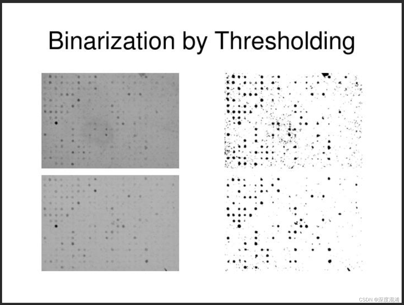
图像阈值分割---迭代算法

(1) 为全局阈值选择一个初始估计值T(图像的平均灰度)。
(2) 用T分割图像。产生两组像素：G1有灰度值大于T的像素组成，G2有小于等于T像素组成。
(3) 计算G1和G2像素的平均灰度值m1和m2；
(4) 计算一个新的阈值:T = (m1 + m2) / 2;
(5) 重复步骤2和4,直到连续迭代中的T值间的差小于一个预定义参数为止。
 

二值算法综述请阅读：

C#，图像二值化（01）——二值化算法综述与二十三种算法目录https://blog.csdn.net/beijinghorn/article/details/128425225?spm=1001.2014.3001.5502

支持函数请阅读：

C#，图像二值化（02）——用于图像二值化处理的一些基本图像处理函数之C#源代码https://blog.csdn.net/beijinghorn/article/details/128425984?spm=1001.2014.3001.5502

2、全局阈值的迭代算法的C#源程序

using System;
using System.Linq;
using System.Text;
using System.Drawing;
using System.Collections;
using System.Collections.Generic;
using System.Runtime.InteropServices;
using System.Drawing.Imaging;

namespace Legalsoft.Truffer.ImageTools
{
    public static partial class BinarizationHelper
    {

        #region 灰度图像二值化 全局算法 迭代算法

        /// <summary>
        /// 阀值分割：迭代法
        /// https://blog.csdn.net/xw20084898/article/details/17564957
        /// </summary>
        /// <param name="data"></param>
        /// <param name="nMaxIter">最大迭代次数</param>
        /// <param name="iDiffRec">使用给定阀值确定的亮区与暗区平均灰度差异值</param>
        /// <returns></returns>
        private static int Iteration_Threshold(byte[,] data, int nMaxIter, out int iDiffRec)
        {
            int height = data.GetLength(0);
            int width = data.GetLength(1);

            iDiffRec = 0;

            int[] histogram = Gray_Histogram(data);
            int iMinGrayValue = Histogram_Left(histogram);
            int iMaxGrayValue = Histogram_Right(histogram);

            int iThrehold = 0;
            int iTotalGray = 0;
            int iTotalPixel = 0;
            int iNewThrehold = (iMinGrayValue + iMaxGrayValue) / 2;
            iDiffRec = iMaxGrayValue - iMinGrayValue;

            for (int a = 0; (Math.Abs(iThrehold - iNewThrehold) > 0.5) && a < nMaxIter; a++)
            {
                iThrehold = iNewThrehold;
                for (int i = iMinGrayValue; i < iThrehold; i++)
                {
                    iTotalGray += histogram[i] * i;
                    iTotalPixel += histogram[i];
                }
                int iMeanGrayValue1 = (iTotalGray / iTotalPixel);
                iTotalPixel = 0;
                iTotalGray = 0;
                for (int j = iThrehold + 1; j < iMaxGrayValue; j++)
                {
                    iTotalGray += histogram[j] * j;
                    iTotalPixel += histogram[j];
                }
                int iMeanGrayValue2 = (iTotalGray / iTotalPixel);

                iNewThrehold = (iMeanGrayValue2 + iMeanGrayValue1) / 2;
                iDiffRec = Math.Abs(iMeanGrayValue2 - iMeanGrayValue1);
            }

            return iThrehold;
        }

        public static void Iteration_Algorithm(byte[,] data)
        {
            int threshold = Iteration_Threshold(data, 100, out int iDiffRec);
            Threshold_Algorithm(data, threshold);
        }

        #endregion

    }
}

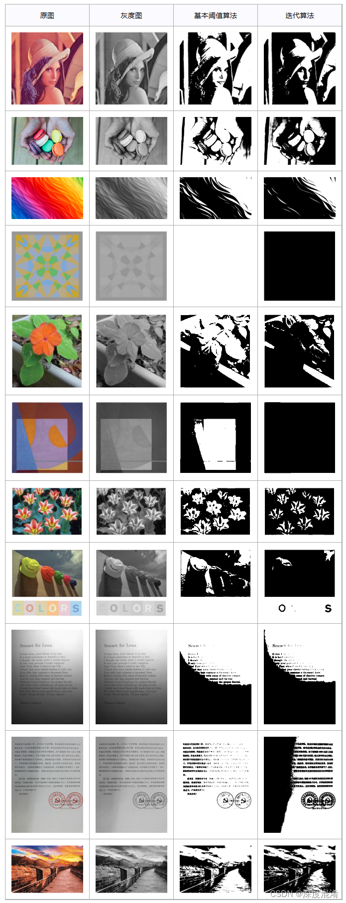
3、全局阈值的迭代算法的计算效果

Image threshold segmentation iterative algorithm

(1) Select an initial estimate T (the average gray level of the image) for the global threshold.

(2) Use T to segment the image. Two groups of pixels are generated: G1 consists of pixels with a gray value greater than T, and G2 consists of pixels with a gray value less than or equal to T.

(3) Calculate the average gray value m1 and m2 of G1 and G2 pixels;

(4) Calculate a new threshold: T=(m1+m2)/2;

(5) Repeat steps 2 and 4 until the difference between T values in successive iterations is less than a predefined parameter.

An iterative algorithm is the most common way to solve the data flow analysis equations. In this algorithm, we particularly have two states first one is in-state and the other one is out-state. The algorithm starts with an approximation of the in-state of each block and then computed by applying the transfer functions on the in-states.

Iterative algorithms (IA) of solving the inverse problems of the scalar theory of diffraction for the calculation of the DOEs, investigated in this section, do not cover the entire spectrum of the currently available iterative algorithms. No attention has been given to algorithms such as the method of direct stochastic search for the binary phase [49], the annealing modelling method [51], the error diffusion method [88], the Newton method for calculating the Dammann gratings [58], and others. These methods are less efficient in comparison with the parametric and gradient iterative algorithms investigated in this chapter, although they are characterised by convergence and reach a global minimum after a large number of iterations.

Although the IAs of the calculating DOEs have shortcomings (for example, the stagnation effect, i.e., as a result of the incorrect selection of the initial estimate of the sought DOE phase, the algorithm can reached a local minimum when the error does not change with the increase of the number of iterations), the obvious advantages of the IA explain why they are used widely in diffractive optics. Some of the advantages of the IA are described below.