Regularized Linear Regression and Bias v.s. Variance

1. Regularized Linear Regression

（1）Visualizing the dataset

ex5.m

%% Machine Learning Online Class
%  Exercise 5 | Regularized Linear Regression and Bias-Variance
%
%  Instructions
%  ------------
% 
%  This file contains code that helps you get started on the
%  exercise. You will need to complete the following functions:
%
%     linearRegCostFunction.m
%     learningCurve.m
%     validationCurve.m
%
%  For this exercise, you will not need to change any code in this file,
%  or any other files other than those mentioned above.
%

%% Initialization
clear ; close all; clc

%% =========== Part 1: Loading and Visualizing Data =============
%  We start the exercise by first loading and visualizing the dataset. 
%  The following code will load the dataset into your environment and plot
%  the data.
%

% Load Training Data
fprintf('Loading and Visualizing Data ...\n')

% Load from ex5data1: 
% You will have X, y, Xval, yval, Xtest, ytest in your environment
load ('ex5data1.mat');

% m = Number of examples
m = size(X, 1);

% Plot training data
plot(X, y, 'rx', 'MarkerSize', 10, 'LineWidth', 1.5);
xlabel('Change in water level (x)');
ylabel('Water flowing out of the dam (y)');

% fprintf('Program paused. Press enter to continue.\n');
% pause;

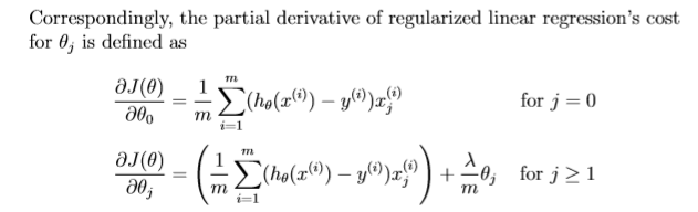
（2）Regularized linear regression

LinearRegCostFunction.m

function [J, grad] = linearRegCostFunction(X, y, theta, lambda)
%LINEARREGCOSTFUNCTION Compute cost and gradient for regularized linear 
%regression with multiple variables
%   [J, grad] = LINEARREGCOSTFUNCTION(X, y, theta, lambda) computes the 
%   cost of using theta as the parameter for linear regression to fit the 
%   data points in X and y. Returns the cost in J and the gradient in grad

% Initialize some useful values
m = length(y); % number of training examples

% You need to return the following variables correctly 
J = 0;
grad = zeros(size(theta));

% ====================== YOUR CODE HERE ======================
% Instructions: Compute the cost and gradient of regularized linear 
%               regression for a particular choice of theta.
%
%               You should set J to the cost and grad to the gradient.
%

h = X * theta;
theta(1) = 0;       % theta_0不惩罚

regTerm = lambda / (2 * m) .* theta' * theta;
J = 1 / (2 * m) .* (h - y)' * (h - y) + regTerm;

grad = 1 / m .* X' * (h - y) + lambda / m .* theta;
grad(1) = grad(1) - lambda / m .* theta(1);

% =========================================================================

grad = grad(:);

end

ex5.m

%% =========== Part 2: Regularized Linear Regression Cost =============
%  You should now implement the cost function for regularized linear 
%  regression. 
%

theta = [1 ; 1];
J = linearRegCostFunction([ones(m, 1) X], y, theta, 1);

fprintf(['Cost at theta = [1 ; 1]: %f '...
         '\n(this value should be about 303.993192)\n'], J);

% fprintf('Program paused. Press enter to continue.\n');
% pause;

（3）Regularized linear regression

LinearRegCostFunction.m

function [J, grad] = linearRegCostFunction(X, y, theta, lambda)
%LINEARREGCOSTFUNCTION Compute cost and gradient for regularized linear 
%regression with multiple variables
%   [J, grad] = LINEARREGCOSTFUNCTION(X, y, theta, lambda) computes the 
%   cost of using theta as the parameter for linear regression to fit the 
%   data points in X and y. Returns the cost in J and the gradient in grad

% Initialize some useful values
m = length(y); % number of training examples

% You need to return the following variables correctly 
J = 0;
grad = zeros(size(theta));

% ====================== YOUR CODE HERE ======================
% Instructions: Compute the cost and gradient of regularized linear 
%               regression for a particular choice of theta.
%
%               You should set J to the cost and grad to the gradient.
%
h = X * theta;
regTerm = lambda / (2 * m) .* theta' * theta;
regTerm(1) = 0;
J = 1 / (2 * m) .* (h - y)' * (h - y) + regTerm;

grad = 1 / m .* X' * (h - y) + lambda / m .* theta;
grad(1) = grad(1) - lambda / m .* theta(1);

% =========================================================================

grad = grad(:);

end

ex5.m

%% =========== Part 3: Regularized Linear Regression Gradient =============
%  You should now implement the gradient for regularized linear 
%  regression.
%

theta = [1 ; 1];
[J, grad] = linearRegCostFunction([ones(m, 1) X], y, theta, 1);

fprintf(['Gradient at theta = [1 ; 1]:  [%f; %f] '...
         '\n(this value should be about [-15.303016; 598.250744])\n'], ...
         grad(1), grad(2));

% fprintf('Program paused. Press enter to continue.\n');
% pause;

（5）Fitting Linear regression

trainLinearReg.m

function [theta] = trainLinearReg(X, y, lambda)
%TRAINLINEARREG Trains linear regression given a dataset (X, y) and a
%regularization parameter lambda
%   [theta] = TRAINLINEARREG (X, y, lambda) trains linear regression using
%   the dataset (X, y) and regularization parameter lambda. Returns the
%   trained parameters theta.
%

% Initialize Theta
initial_theta = zeros(size(X, 2), 1); 

% Create "short hand" for the cost function to be minimized
costFunction = @(t) linearRegCostFunction(X, y, t, lambda);

% Now, costFunction is a function that takes in only one argument
options = optimset('MaxIter', 200, 'GradObj', 'on');

% Minimize using fmincg
theta = fmincg(costFunction, initial_theta, options);

end

ex5.m

%% =========== Part 4: Train Linear Regression =============
%  Once you have implemented the cost and gradient correctly, the
%  trainLinearReg function will use your cost function to train 
%  regularized linear regression.
% 
%  Write Up Note: The data is non-linear, so this will not give a great 
%                 fit.
%

%  Train linear regression with lambda = 0
lambda = 0;
[theta] = trainLinearReg([ones(m, 1) X], y, lambda);

%  Plot fit over the data
plot(X, y, 'rx', 'MarkerSize', 10, 'LineWidth', 1.5);
xlabel('Change in water level (x)');
ylabel('Water flowing out of the dam (y)');
hold on;
plot(X, [ones(m, 1) X]*theta, '--', 'LineWidth', 2)
hold off;

% fprintf('Program paused. Press enter to continue.\n');
% pause;

2. Bias-variance

（1）Learning curves

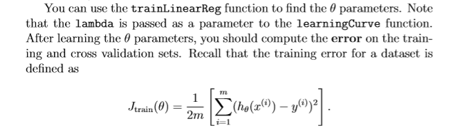
注意：训练误差并不包含正则化项。计算训练误差的一种方法是使用现有的代价函数，仅当使用它来计算训练误差和交叉验证误差时，将 λ 设置为0。 当你正在计算训练误差时，要确保在训练子集上计算训练误差，而不是在整个训练集上计算。但是，当你在计算交叉验证误差时，你应该在整个交叉验证集上计算它。
learningCurve.m

function [error_train, error_val] = ...
    learningCurve(X, y, Xval, yval, lambda)
%LEARNINGCURVE Generates the train and cross validation set errors needed 
%to plot a learning curve
%   [error_train, error_val] = ...
%       LEARNINGCURVE(X, y, Xval, yval, lambda) returns the train and
%       cross validation set errors for a learning curve. In particular, 
%       it returns two vectors of the same length - error_train and 
%       error_val. Then, error_train(i) contains the training error for
%       i examples (and similarly for error_val(i)).
%
%   In this function, you will compute the train and test errors for
%   dataset sizes from 1 up to m. In practice, when working with larger
%   datasets, you might want to do this in larger intervals.
%

% Number of training examples
m = size(X, 1);

% You need to return these values correctly
error_train = zeros(m, 1);
error_val   = zeros(m, 1);

% ====================== YOUR CODE HERE ======================
% Instructions: Fill in this function to return training errors in 
%               error_train and the cross validation errors in error_val. 
%               i.e., error_train(i) and 
%               error_val(i) should give you the errors
%               obtained after training on i examples.
%
% Note: You should evaluate the training error on the first i training
%       examples (i.e., X(1:i, :) and y(1:i)).
%
%       For the cross-validation error, you should instead evaluate on
%       the _entire_ cross validation set (Xval and yval).
%
% Note: If you are using your cost function (linearRegCostFunction)
%       to compute the training and cross validation error, you should 
%       call the function with the lambda argument set to 0. 
%       Do note that you will still need to use lambda when running
%       the training to obtain the theta parameters.
%
% Hint: You can loop over the examples with the following:
%
%       for i = 1:m
%           % Compute train/cross validation errors using training examples 
%           % X(1:i, :) and y(1:i), storing the result in 
%           % error_train(i) and error_val(i)
%           ....
%           
%       end
%

% ---------------------- Sample Solution ----------------------

for i = 1 : m
    theta = trainLinearReg(X(1:i, :), y(1:i, :), lambda);
    error_train(i) = linearRegCostFunction(X(1:i, :), y(1:i, :), theta, 0);
    error_val(i) = linearRegCostFunction(Xval, yval, theta, 0);
end

% -------------------------------------------------------------

% =========================================================================

end

ex5.m

%% =========== Part 5: Learning Curve for Linear Regression =============
%  Next, you should implement the learningCurve function. 
%
%  Write Up Note: Since the model is underfitting the data, we expect to
%                 see a graph with "high bias" -- Figure 3 in ex5.pdf 
%

lambda = 0;
[error_train, error_val] = ...
    learningCurve([ones(m, 1) X], y, ...
                  [ones(size(Xval, 1), 1) Xval], yval, ...
                  lambda);

plot(1:m, error_train, 1:m, error_val);
title('Learning curve for linear regression')
legend('Train', 'Cross Validation')
xlabel('Number of training examples')
ylabel('Error')
axis([0 13 0 150])

fprintf('# Training Examples\tTrain Error\tCross Validation Error\n');
for i = 1:m
    fprintf('  \t%d\t\t%f\t%f\n', i, error_train(i), error_val(i));
end

% fprintf('Program paused. Press enter to continue.\n');
% pause;

3. Polynomial regression

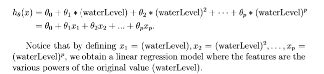
polyFeatures.m

function [X_poly] = polyFeatures(X, p)
%POLYFEATURES Maps X (1D vector) into the p-th power
%   [X_poly] = POLYFEATURES(X, p) takes a data matrix X (size m x 1) and
%   maps each example into its polynomial features where
%   X_poly(i, :) = [X(i) X(i).^2 X(i).^3 ...  X(i).^p];
%


% You need to return the following variables correctly.
X_poly = zeros(numel(X), p);

% ====================== YOUR CODE HERE ======================
% Instructions: Given a vector X, return a matrix X_poly where the p-th 
%               column of X contains the values of X to the p-th power.
%
% 

for i = 1:p
    X_poly(:,i) = X.^i;    
end



% =========================================================================

end

（1） Learning Polynomial Regression

归一化处理
$$\frac{x_i-\mu }{\sqrt{\sigma }}$$
其中 $\mu$ 表示均值，$\sigma$ 表示方差

featureNormalize.m

function [X_norm, mu, sigma] = featureNormalize(X)
%FEATURENORMALIZE Normalizes the features in X 
%   FEATURENORMALIZE(X) returns a normalized version of X where
%   the mean value of each feature is 0 and the standard deviation
%   is 1. This is often a good preprocessing step to do when
%   working with learning algorithms.

mu = mean(X);
X_norm = bsxfun(@minus, X, mu);

sigma = std(X_norm);
X_norm = bsxfun(@rdivide, X_norm, sigma);


% ============================================================

end

ex5.m

%% =========== Part 6: Feature Mapping for Polynomial Regression =============
%  One solution to this is to use polynomial regression. You should now
%  complete polyFeatures to map each example into its powers
%

p = 8;

% Map X onto Polynomial Features and Normalize
X_poly = polyFeatures(X, p);
[X_poly, mu, sigma] = featureNormalize(X_poly);  % Normalize
X_poly = [ones(m, 1), X_poly];                   % Add Ones

% Map X_poly_test and normalize (using mu and sigma)
X_poly_test = polyFeatures(Xtest, p);
X_poly_test = bsxfun(@minus, X_poly_test, mu);
X_poly_test = bsxfun(@rdivide, X_poly_test, sigma);
X_poly_test = [ones(size(X_poly_test, 1), 1), X_poly_test];         % Add Ones

% Map X_poly_val and normalize (using mu and sigma)
X_poly_val = polyFeatures(Xval, p);
X_poly_val = bsxfun(@minus, X_poly_val, mu);
X_poly_val = bsxfun(@rdivide, X_poly_val, sigma);
X_poly_val = [ones(size(X_poly_val, 1), 1), X_poly_val];           % Add Ones

fprintf('Normalized Training Example 1:\n');
fprintf('  %f  \n', X_poly(1, :));

% fprintf('\nProgram paused. Press enter to continue.\n');
% pause;

绘制曲线
plotFit.m

function plotFit(min_x, max_x, mu, sigma, theta, p)
%PLOTFIT Plots a learned polynomial regression fit over an existing figure.
%Also works with linear regression.
%   PLOTFIT(min_x, max_x, mu, sigma, theta, p) plots the learned polynomial
%   fit with power p and feature normalization (mu, sigma).

% Hold on to the current figure
hold on;

% We plot a range slightly bigger than the min and max values to get
% an idea of how the fit will vary outside the range of the data points
x = (min_x - 15: 0.05 : max_x + 25)';

% Map the X values 
X_poly = polyFeatures(x, p);
X_poly = bsxfun(@minus, X_poly, mu);
X_poly = bsxfun(@rdivide, X_poly, sigma);

% Add ones
X_poly = [ones(size(x, 1), 1) X_poly];

% Plot
plot(x, X_poly * theta, '--', 'LineWidth', 2)

% Hold off to the current figure
hold off

end

ex5.m

%% =========== Part 7: Learning Curve for Polynomial Regression =============
%  Now, you will get to experiment with polynomial regression with multiple
%  values of lambda. The code below runs polynomial regression with 
%  lambda = 0. You should try running the code with different values of
%  lambda to see how the fit and learning curve change.
%

lambda = 0;
[theta] = trainLinearReg(X_poly, y, lambda);

% Plot training data and fit
figure(1);
plot(X, y, 'rx', 'MarkerSize', 10, 'LineWidth', 1.5);
plotFit(min(X), max(X), mu, sigma, theta, p);
xlabel('Change in water level (x)');
ylabel('Water flowing out of the dam (y)');
title (sprintf('Polynomial Regression Fit (lambda = %f)', lambda));

figure(2);
[error_train, error_val] = ...
    learningCurve(X_poly, y, X_poly_val, yval, lambda);
plot(1:m, error_train, 1:m, error_val);

title(sprintf('Polynomial Regression Learning Curve (lambda = %f)', lambda));
xlabel('Number of training examples')
ylabel('Error')
axis([0 13 0 100])
legend('Train', 'Cross Validation')

fprintf('Polynomial Regression (lambda = %f)\n\n', lambda);
fprintf('# Training Examples\tTrain Error\tCross Validation Error\n');
for i = 1:m
    fprintf('  \t%d\t\t%f\t%f\n', i, error_train(i), error_val(i));
end

% fprintf('Program paused. Press enter to continue.\n');
% pause;

$\lambda =0$ 时，


$\lambda =1$ 时，你应该会看到一个多项式拟合，它很好地拟合了数据趋势(图6)和一个学习曲线(图7)，该曲线表明交叉验证和训练误差都收敛到一个相对较低的值。 这表明λ = 1正则化多项式回归模型不存在高偏差或高方差问题。 实际上，它在偏差和方差之间取得了很好的平衡。


$\lambda =100$ 时，你应该会看到一个不符合数据的多项式拟合(图8)。 这种情况下正则化过多，模型无法拟合训练数据。

（3） Selecting λ using a cross validation set

validationCurve.m

function [lambda_vec, error_train, error_val] = ...
    validationCurve(X, y, Xval, yval)
%VALIDATIONCURVE Generate the train and validation errors needed to
%plot a validation curve that we can use to select lambda
%   [lambda_vec, error_train, error_val] = ...
%       VALIDATIONCURVE(X, y, Xval, yval) returns the train
%       and validation errors (in error_train, error_val)
%       for different values of lambda. You are given the training set (X,
%       y) and validation set (Xval, yval).
%

% Selected values of lambda (you should not change this)
lambda_vec = [0 0.001 0.003 0.01 0.03 0.1 0.3 1 3 10]';

% You need to return these variables correctly.
error_train = zeros(length(lambda_vec), 1);
error_val = zeros(length(lambda_vec), 1);

% ====================== YOUR CODE HERE ======================
% Instructions: Fill in this function to return training errors in 
%               error_train and the validation errors in error_val. The 
%               vector lambda_vec contains the different lambda parameters 
%               to use for each calculation of the errors, i.e, 
%               error_train(i), and error_val(i) should give 
%               you the errors obtained after training with 
%               lambda = lambda_vec(i)
%
% Note: You can loop over lambda_vec with the following:
%
%       for i = 1:length(lambda_vec)
%           lambda = lambda_vec(i);
%           % Compute train / val errors when training linear 
%           % regression with regularization parameter lambda
%           % You should store the result in error_train(i)
%           % and error_val(i)
%           ....
%           
%       end
%
%

for i = 1 : length(lambda_vec)
    lambda = lambda_vec(i);
    theta = trainLinearReg(X, y, lambda);
    error_train(i) = linearRegCostFunction(X, y, theta, 0);
    error_val(i) = linearRegCostFunction(Xval, yval, theta, 0);    
end






% =========================================================================

end

ex5.m

%% =========== Part 8: Validation for Selecting Lambda =============
%  You will now implement validationCurve to test various values of 
%  lambda on a validation set. You will then use this to select the
%  "best" lambda value.
%

[lambda_vec, error_train, error_val] = ...
    validationCurve(X_poly, y, X_poly_val, yval);

close all;
plot(lambda_vec, error_train, lambda_vec, error_val);
legend('Train', 'Cross Validation');
xlabel('lambda');
ylabel('Error');

fprintf('lambda\t\tTrain Error\tValidation Error\n');
for i = 1:length(lambda_vec)
	fprintf(' %f\t%f\t%f\n', ...
            lambda_vec(i), error_train(i), error_val(i));
end

% fprintf('Program paused. Press enter to continue.\n');
% pause;

通过图中曲线可发现， $\lambda$ 取3时最佳。绘制代价曲线误差如下

全部作业代码

MLExercise_Ng