目录

1.算法描述

2.仿真效果预览

3.MATLAB部分代码预览

4.完整MATLAB程序

1.算法描述

       CT重建算法大致分为解析重建算法和迭代重建算法，随着CT技术的发展，重建算法也变得多种多样，各有各的有特点。本文使用目前应用最广泛的重建算法——滤波反投影算法（FBP）作为模型的基础算法。FBP算法是在傅立叶变换理论基础之上的一种空域处理技术。它的特点是在反投影前将每一个采集投影角度下的投影进行卷积处理，从而改善点扩散函数引起的形状伪影，重建的图像质量较好。

       上图应可以清晰的描述傅立叶中心切片定理的过程：对投影的一维傅立叶变换等效于对原图像进行二维的傅立叶变换。傅立叶切片定理的意义在于，通过投影上执行傅立叶变换，可以从每个投影中得到二维傅立叶变换。从而投影图像重建的问题，可以按以下方法进行求解：采集不同时间下足够多的投影（一般为180次采集），求解各个投影的一维傅立叶变换，将上述切片汇集成图像的二维傅立叶变换，再利用傅立叶反变换求得重建图像。

       投影重建的过程是，先把投影由线阵探测器上获得的投影数据进行一次一维傅立叶变换，再与滤波器函数进行卷积运算，得到各个方向卷积滤波后的投影数据；然后把它们沿各个方向进行反投影，即按其原路径平均分配到每一矩阵单元上，进行重叠后得到每一矩阵单元的CT值；再经过适当处理后得到被扫描物体的断层图像
算法步骤如下：
1. 将原始投影进行一次一维傅立叶变换
2. 设计合适的滤波器，在φ_i的角度下将得到原始投影p(x_r,φ_i)进行卷积滤波，得到滤波后的投影。
3. 将滤波后的投影进行反投影，得到满足x_r=r cos⁡（(θ - φ_i)）方向上的原图像的密度。
4. 将所有反投影进行叠加，得到重建后的投影。 

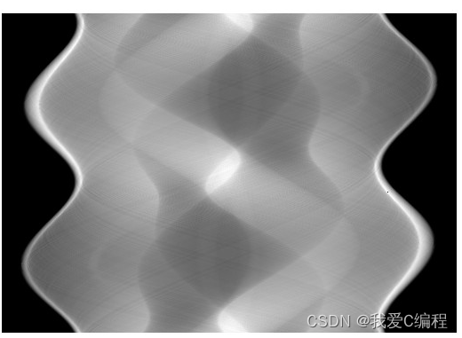
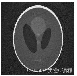
2.仿真效果预览

matlab2013B仿真结果如下：

3.MATLAB部分代码预览

coordinateSource=[];
projMatrix=[];
detector=[];
proj=load(char('projection.mat'));
phyRatoDig=proj.phyRatoDig;
projMatrix=proj.projection;
yDetector=proj.yDetector;
nDetectors=proj.nDetectors;
 
figure(2)
showimge(projMatrix,360,512,0,max(max(projMatrix)));
 
 
D_dig=proj.focalDistance_dig;
sourceToDetector_dig=proj.focalDistance_dig+proj.detecDistance_dig;
s=[];
s=D_dig/sourceToDetector_dig*yDetector(1,:)*phyRatoDig;
Detector=yDetector(1,:)*phyRatoDig;
% 
 pe=[];
 M=D_dig./sqrt(D_dig.^2+s.^2);
 nViews=proj.nViews;
% 
 for i=1:nViews
    pe(i,:)=projMatrix(i,:).*M;
     
 end
 figure(3);
 showimge(pe,360,512,0,max(max(pe)));
 
 
 
disp('Filtering')
filternum=128;
filter_ramp=zeros(filternum,1);
for j=1:filternum   % 16 point ramp filter
    i=j-1-filternum/2;
    if(i==0)
     filter_ramp(j,1)=1/(8.0);
    elseif (mod(i,2)==0)
            filter_ramp(j,1)=0;
    elseif (mod(i,2)==1)
            filter_ramp(j,1)=-0.5/(i*i*pi*pi);
    end
end
m=1;
figure(4);
 
plot(filter_ramp);
 
 
pfilter=[];
length_conv=filternum+nDetectors-1;
pPro=zeros(length_conv,1);
temp_pro=zeros(nDetectors,1);
h_filter=filternum/2;
ii=length_conv-h_filter-nDetectors;
 for s=1:nViews % sample-loop
    % for  pp=1:h_filter
    pro_left =(pe(s,1)+pe(s,2))/2.0;
    pro_right=(pe(s,nDetectors)+pe(s,nDetectors-1))/2.0;
    
    for pp=1:h_filter;               %left part
        pPro(pp,1)=pro_left;        
    end
%    
    for pp=1:nDetectors                      %middle part
     pPro(h_filter+pp,1)=pe(s,pp);
    end
%    
   for pp=h_filter+nDetectors+1:length_conv
    pPro(pp)=pro_right;
    end
%   result_conv    
   for n=1:nDetectors 
       result_conv=0;
   	for jj=1:filternum
        pPmove=pPro(n+jj-1,1);
        result_conv=result_conv+pPmove*filter_ramp(jj,1);
    end
    pfilter(s,n)=result_conv;
   end
 
    
 end
figure(5);
showimge(pfilter,360,512,min(min(pfilter)),max(max(pfilter)));
 
% %%%%%%%%%%%%%%%%%%%%%%reArrange%%%%%%%%%%%%%%%%%%%%%%%%%%%%%%%%%%%
% %%%%%%%%%%%%%%%%%%%%%%Back projection%%%%%%%%%%%%%%%%%%%%%%%%%%%%%
disp('BackProjection')
detecLength=proj.detecLength;
unitDis=detecLength/(nDetectors-1);
unitDis_dig=unitDis*phyRatoDig;
deltaBeta=2*pi/nViews;
 M=proj.M;
 N=proj.N;
 fReconstruct=[];
 for i=1:M
      x=i-(M+1)/2;
     for j=1:N
        y=(N+1)/2-j;
       r=sqrt(x^2+y^2);
        theta=atan2(y,x);
%     
        result=0; 
     for s=1:nViews
     beta= (s-1)*deltaBeta;
     s1=D_dig*r*cos(beta-theta)/(D_dig+r*sin(beta-theta));
     U=(D_dig+r*sin(beta-theta))/D_dig;
     p1=sourceToDetector_dig/D_dig*s1;
     if(p1>Detector(1,1)&&p1<Detector(1,512))
         num=(p1-Detector(1,1)+unitDis_dig)/unitDis_dig;        
         numlow=floor(num);
         result=result+((num-numlow)*pfilter(s,numlow)+(1-num+numlow)*pfilter(s,numlow+1))/U/U*deltaBeta;
     end
     end
     fReconstruct(i,j)=result;
     if( fReconstruct(i,j)<0)
         fReconstruct(i,j)=0;
     end
 
     end
 end
% 
 figure(6)
% 
final=zeros(M,N);
for i=1:M
    final(i,:)=fReconstruct(:,257-i);
end
A_022

4.完整MATLAB程序

matlab源码说明_我爱C编程的博客-CSDN博客

V