
[Intro to Deep Learning with PyTorch -- L2 -- N9] Perceptron Trick
Give this:
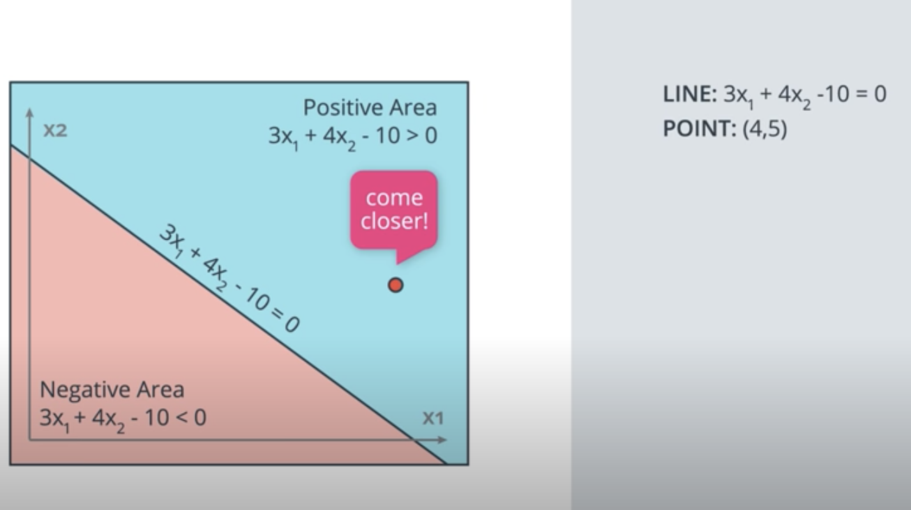
We have a wrongn classified point, how to move the line to come closer to the points?

We apply learning rate and since wrong point is in positive area, we need to W - learning rate * wrong cord
The same, if the wrong point in negivate area, we do : W + learing rate * wrong cord:
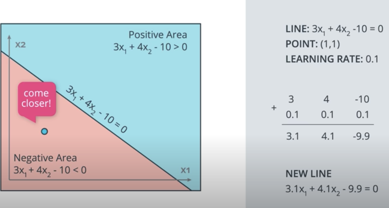
For the second example, where the line is described by 3x1+ 4x2 - 10 = 0, if the learning rate was set to 0.1, how many times would you have to apply the perceptron trick to move the line to a position where the blue point, at (1, 1), is correctly classified?
Answer: 10 times
Coding the Perceptron Algorithm
Time to code! In this quiz, you'll have the chance to implement the perceptron algorithm to separate the following data (given in the file data.csv).

Recall that the perceptron step works as follows. For a point with coordinates (p,q)(p,q), label yy, and prediction given by the equation \hat{y} = step(w_1x_1 + w_2x_2 + b)y^=step(w1x1+w2x2+b):
- If the point is correctly classified, do nothing.
- If the point is classified positive, but it has a negative label, subtract \alpha p, \alpha q,αp,αq, and \alphaα from w_1, w_2,w1,w2, and bb respectively.
- If the point is classified negative, but it has a positive label, add \alpha p, \alpha q,αp,αq, and \alphaα to w_1, w_2,w1,w2, and bb respectively.
Then click on test run to graph the solution that the perceptron algorithm gives you. It'll actually draw a set of dotted lines, that show how the algorithm approaches to the best solution, given by the black solid line.
import numpy as np
# Setting the random seed, feel free to change it and see different solutions.
np.random.seed(42)

def stepFunction(t):
    if t >= 0:
        return 1
    return 0

def prediction(X, W, b):
    return stepFunction((np.matmul(X,W)+b)[0])

# TODO: Fill in the code below to implement the perceptron trick.
# The function should receive as inputs the data X, the labels y,
# the weights W (as an array), and the bias b,
# update the weights and bias W, b, according to the perceptron algorithm,
# and return W and b.
def perceptronStep(X, y, W, b, learn_rate = 0.01):
    for i in range(len(X)):
        y_hat = prediction(X[i], W, b)
        # predition in prostive area
        if y[i]-y_hat == -1:
            W[0] -= X[i][0]*learn_rate
            W[1] -= X[i][1]*learn_rate
            b -= learn_rate
        # predition in negivate area
        elif y[i]-y_hat == 1:
            W[0] += X[i][0]*learn_rate
            W[1] += X[i][1]*learn_rate
            b += learn_rate

    return W, b

# This function runs the perceptron algorithm repeatedly on the dataset,
# and returns a few of the boundary lines obtained in the iterations,
# for plotting purposes.
# Feel free to play with the learning rate and the num_epochs,
# and see your results plotted below.
def trainPerceptronAlgorithm(X, y, learn_rate = 0.01, num_epochs = 25):
    x_min, x_max = min(X.T[0]), max(X.T[0])
    y_min, y_max = min(X.T[1]), max(X.T[1])
    W = np.array(np.random.rand(2,1))
    b = np.random.rand(1)[0] + x_max
    # These are the solution lines that get plotted below.
    boundary_lines = []
    for i in range(num_epochs):
        # In each epoch, we apply the perceptron step.
        W, b = perceptronStep(X, y, W, b, learn_rate)
        boundary_lines.append((-W[0]/W[1], -b/W[1]))
    return boundary_lines
0.78051,-0.063669,1
0.28774,0.29139,1
0.40714,0.17878,1
0.2923,0.4217,1
0.50922,0.35256,1
0.27785,0.10802,1
0.27527,0.33223,1
0.43999,0.31245,1
0.33557,0.42984,1
0.23448,0.24986,1
0.0084492,0.13658,1
0.12419,0.33595,1
0.25644,0.42624,1
0.4591,0.40426,1
0.44547,0.45117,1
0.42218,0.20118,1
0.49563,0.21445,1
0.30848,0.24306,1
0.39707,0.44438,1
0.32945,0.39217,1
0.40739,0.40271,1
0.3106,0.50702,1
0.49638,0.45384,1
0.10073,0.32053,1
0.69907,0.37307,1
0.29767,0.69648,1
0.15099,0.57341,1
0.16427,0.27759,1
0.33259,0.055964,1
0.53741,0.28637,1
0.19503,0.36879,1
0.40278,0.035148,1
0.21296,0.55169,1
0.48447,0.56991,1
0.25476,0.34596,1
0.21726,0.28641,1
0.67078,0.46538,1
0.3815,0.4622,1
0.53838,0.32774,1
0.4849,0.26071,1
0.37095,0.38809,1
0.54527,0.63911,1
0.32149,0.12007,1
0.42216,0.61666,1
0.10194,0.060408,1
0.15254,0.2168,1
0.45558,0.43769,1
0.28488,0.52142,1
0.27633,0.21264,1
0.39748,0.31902,1
0.5533,1,0
0.44274,0.59205,0
0.85176,0.6612,0
0.60436,0.86605,0
0.68243,0.48301,0
1,0.76815,0
0.72989,0.8107,0
0.67377,0.77975,0
0.78761,0.58177,0
0.71442,0.7668,0
0.49379,0.54226,0
0.78974,0.74233,0
0.67905,0.60921,0
0.6642,0.72519,0
0.79396,0.56789,0
0.70758,0.76022,0
0.59421,0.61857,0
0.49364,0.56224,0
0.77707,0.35025,0
0.79785,0.76921,0
0.70876,0.96764,0
0.69176,0.60865,0
0.66408,0.92075,0
0.65973,0.66666,0
0.64574,0.56845,0
0.89639,0.7085,0
0.85476,0.63167,0
0.62091,0.80424,0
0.79057,0.56108,0
0.58935,0.71582,0
0.56846,0.7406,0
0.65912,0.71548,0
0.70938,0.74041,0
0.59154,0.62927,0
0.45829,0.4641,0
0.79982,0.74847,0
0.60974,0.54757,0
0.68127,0.86985,0
0.76694,0.64736,0
0.69048,0.83058,0
0.68122,0.96541,0
0.73229,0.64245,0
0.76145,0.60138,0
0.58985,0.86955,0
0.73145,0.74516,0
0.77029,0.7014,0
0.73156,0.71782,0
0.44556,0.57991,0
0.85275,0.85987,0
0.51912,0.62359,0

相关文章
- [Intro to Deep Learning with PyTorch -- L2 -- N15] Softmax function
- [Intro to Deep Learning with PyTorch -- L2 -- N14] Sigmoid function
- 机器学习笔记 - Pytorch要点和实现MNIST分类
- 【PyTorch】教程:torch.nn.CELU
- 【PyTorch】教程:对抗学习实例生成
- 【PyTorch】教程:学习基础知识-(3) Datasets-DataLoader
- DL:深度学习框架Pytorch、 Tensorflow各种角度对比
- AutoMl 的pytorch类似代码
- PyTorch存储和加载模型并查看参数,load_state_dict(),state_dict() + 使用多张GPU进行训练以及推理调用模型
- 【NLP】使用递归神经网络对序列数据进行建模 (Pytorch)
- 【Pytorch深度学习实战】(6)递归神经网络(RNN)
- Pytorch 实现逻辑回归
- 赶快收藏:快速安装PyTorch和TensorFlow(gpu+cpu+1.7.1+2.2.0--cuda_11.0.2_450.51.05)命令
- 【Deepin 20系统】Linux系统安装Pytorch、Torch
- pytorch中的unsqueeze()函数解析
- Pytorch总结十四之优化算法:梯度下降法、动量法
- Pytorch总结八之深度学习计算(1)模型构造,参数访问、初始化和共享
- 【Pytorch Lighting】第 7 章:半监督学习