Evaluating a Hypothesis

1. Evaluating a Learning Algorithm

（1） Evaluating a Hypothesis

Once we have done some trouble shooting for errors in our predictions by:

• Getting more training examples

• Trying smaller sets of features

• Trying additional features

• Trying polynomial features

• Increasing or decreasing λ

A hypothesis may have a low error for the training examples but still be inaccurate (because of overfitting). Thus, to evaluate a hypothesis, given a dataset of training examples, we can split up the data into two sets: a training set and a test set. Typically, the training set consists of 70 % of your data and the test set is the remaining 30 %.

The new procedure using these two sets is then:

1. Learn $\Theta$ and minimize $J_{train}(\Theta )$ using the training set
2. Compute the test set error $J_{test}(\Theta )$

The test set error

1. For linear regression : $J_{test}(\Theta )=\frac{1}{2m_{test}}{\sum }_{i=1}^{m_{test}}(h_{\Theta }(x_{test}^{(i)})-(y_{test}^{(i)}){)}^2$
2. For classification ~ Misclassification error(aka 0/1 misclassification error):
   $$err(h_{\Theta }(x),y)=\{\begin{array}{rl}& 1if{h}_{\Theta }(x)\ge 0.5andy=0or{h}_{\Theta }(x)＜0.5andy=1\\ & 0\end{array}$$

This gives us a binary 0 or 1 error result based on a misclassification. The average test error for the test set is:
$$TestError=\frac{1}{m_{test}}\sum _{i=1}^{m_{test}}err(h_{\Theta }(x_{test}^{(i)}),y_{test}^{(i)})$$
This gives us the proportion of the test data that was misclassified.

---

一旦我们通过以下方法解决了预测中的错误:

• 获取更多的训练样例

• 尝试更小的特征集

• 尝试添加更多特征

• 尝试多项式特征

• 增大或减小 λ

一个假设对于训练样例可能有一个很小的误差，但仍然是不准确的(因为过拟合)。因此，为了评估一个假设，给定一个训练样本的数据集，我们可以将数据分成两个集：一个训练集和一个测试集。 通常，训练集包含70%的数据，测试集是剩下的30%的数据。

使用这两个集合的新过程是:

1. 使用训练集数据学习参数 $\Theta$ 并最小化 $J_{train}(\Theta )$
2. 计算测试集的误差 $J_{test}(\Theta )$

测试集错误

1. 对于线性回归 : $J_{test}(\Theta )=\frac{1}{2m_{test}}{\sum }_{i=1}^{m_{test}}(h_{\Theta }(x_{test}^{(i)})-(y_{test}^{(i)}){)}^2$
2. 对于分类 ~ 错误分类误差(又名 0/1 错误分类误差):
   $$err(h_{\Theta }(x),y)=\{\begin{array}{rl}& 1if{h}_{\Theta }(x)\ge 0.5andy=0or{h}_{\Theta }(x)＜0.5andy=1\\ & 0\end{array}$$

这给我们一个基于错误分类的二进制0或1错误结果。 测试集的平均测试误差为:
$$TestError=\frac{1}{m_{test}}\sum _{i=1}^{m_{test}}err(h_{\Theta }(x_{test}^{(i)}),y_{test}^{(i)})$$
这给了我们错误分类的测试数据的比例。

（2）Model Seletction and Train/Validation/Test Sets

Just because a learning algorithm fits a training set well, that does not mean it is a good hypothesis. It could over fit and as a result your predictions on the test set would be poor. The error of your hypothesis as measured on the data set with which you trained the parameters will be lower than the error on any other data set.

Given many models with different polynomial degrees, we can use a systematic approach to identify the ‘best’ function. In order to choose the model of your hypothesis, you can test each degree of polynomial and look at the error result.

One way to break down our dataset into the three sets is:

• Training set: 60%

• Cross validation set: 20%

• Test set: 20%
  
  We can now calculate three separate error values for the three different sets using the following method:

1. Optimize the parameters in Θ using the training set for each polynomial degree.
2. Find the polynomial degree d with the least error using the cross validation set.
3. Estimate the generalization error using the test set with $J_{test}({\Theta }^{(D)})$ (d = theta from polynomial with lower error).

This way, the degree of the polynomial d has not been trained using the test set.

---

仅仅因为一个学习算法很适合一个训练集，并不能说明它是一个好的假设。它可能会过拟合，导致你对测试集的预测结果将会很差。在你训练参数的数据集上测量的假设的误差将低于任何其他数据集上的误差。

给定许多具有不同多项式度的模型，我们可以使用系统的方法来确定“最佳”函数。为了选择你的假设模型，你可以测试每一个多项式的次数，看看错误的结果。

将我们的数据集分解成三个集合的一种方法是：

• 训练集: 60%

• 交叉验证集: 20%

• 测试集: 20%
  

现在我们可以使用以下方法为这三个不同的集合计算三个独立的误差值：

1. 使用训练集中所有多项式不同的次方数来优化 Θ 中的参数。
2. 使用交叉验证集找出误差最小的多项式次方d。
3. 使用测试集$J_{test}({\theta }^{(D)})$ （D = θ来自误差较小的多项式）估计泛化误差。

这样，就没有使用测试集的数据来训练多项式d的次方数。

2. Bias vs. Variance

（1）Diagnosing Bias vs. Variance

In this section we examine the relationship between the degree of the polynomial d and the underfitting or overfitting of our hypothesis.

• We need to distinguish whether bias or variance is the problem contributing to bad predictions.
• High bias is underfitting and high variance is overfitting. Ideally, we need to find a golden mean between these two.

The training error will tend to decrease as we increase the degree d of the polynomial.

At the same time, the cross validation error will tend to decrease as we increase d up to a point, and then it will increase as d is increased, forming a convex curve.

High bias(underfitting): both $J_{train}(\Theta )$ and $J_{CV}(\Theta )$ will be high. Also, $J_{cv}(\Theta )\approx J_{train}(\Theta )$

High variance(overfitting): $J_{train}(\Theta )$ will be low and $J_{CV}(\Theta )$ will be much greater than $J_{train}(\Theta )$

This is summarized in the figure below:

---

在这一节中，我们将检查多项式的次方数d与我们所假设的欠拟合或过拟合之间的关系。

• 我们需要区分到底是偏差还是方差导致了糟糕的预测。
• 高偏差是欠拟合，高方差是过拟合。理想情况下，我们需要在这两者之间找到一个黄金平衡点。

训练误差会随着多项式的d次方树的增加而减少。

同时，交叉验证误差会随着d向一个点处增大时减小，到达这个点之后，随着d的继续增大，交叉验证误差又会增大，最终形成一个凸曲线。

高偏差（欠拟合）: $J_{train}(\Theta )$ 和 $J_{CV}(\Theta )$ 将会很“高”. 同时，$J_{cv}(\Theta )\approx J_{train}(\Theta )$

高方差（多拟合） $J_{train}(\Theta )$将会很低 而 $J_{CV}(\Theta )$ 将会远大于 $J_{train}(\Theta )$（$J_{CV}(\Theta )\gg J_{train}(\Theta$）

下图总结了这一点：

（2）Regularization and Bias/Variance

The regularization term below and through out the video should be $\frac{\lambda }{2m}{\sum }_{j=1}^n{\theta }_j^2$ and NOT $\frac{\lambda }{2m}{\sum }_{j=1}^m{\theta }_j^2$

In the figure above, we see that as \lambdaλ increases, our fit becomes more rigid. On the other hand, as \lambdaλ approaches 0, we tend to over overfit the data. So how do we choose our parameter \lambdaλ to get it ‘just right’ ? In order to choose the model and the regularization term λ, we need to:

1. Create a list of lambdas (i.e. λ∈{0,0.01,0.02,0.04,0.08,0.16,0.32,0.64,1.28,2.56,5.12,10.24});

2. Create a set of models with different degrees or any other variants.

3. Iterate through the \lambdaλs and for each \lambdaλ go through all the models to learn some \ThetaΘ.

4. Compute the cross validation error using the learned Θ (computed with λ) on the $J_{CV}(\Theta )$ without regularization or λ = 0.

5. Select the best combo that produces the lowest error on the cross validation set.

6. Using the best combo Θ and λ, apply it on $J_{test}(\Theta )$ to see if it has a good generalization of the problem.

The regularization term below and through out the video should be $\frac{\lambda }{2m}{\sum }_{j=1}^n{\theta }_j^2$ and NOT $\frac{\lambda }{2m}{\sum }_{j=1}^m{\theta }_j^2$

---

下面和整个视频的正则化项应该是$\frac{\lambda }{2m}{\sum }_{j=1}^n{\theta }_j^2$ 而不是$\frac{\lambda }{2m}{\sum }_{j=1}^m{\theta }_j^2$
在上图中，我们看到随着λ的增加，我们的拟合变得更加严格。另一方面，当λ接近0时，会有过度拟合数据的趋向。 那么我们如何选择我们的参数λ让它“刚刚好呢”？为了选择模型和正则化项λ，我们需要:

1. 创建lambdas的列表(i.e.λ∈{0,0.01,0.02,0.04,0.08,0.16,0.32,0.64,1.28,2.56,5.12,10.24});

2. 创建一组具有不同程度或任何其他变形的模型。

3. 遍历 λ列表，取到每个λ并遍历所有模型来学习一些参数Θ

4. 在没有正则化或λ = 0的情况下，使用学习到的Θ(用λ计算)在$J_{CV}(\theta )$上计算交叉验证误差。

5. 选择在交叉验证集中产生最低错误的最佳组合

6. 使用最好的组合Θ和λ，将它应用到$J_{test}(\Theta )$上，看看它是否有一个很好的泛化能力。

下面和整个视频的正则化项应该是$\frac{\lambda }{2m}{\sum }_{j=1}^n{\theta }_j^2$ 而不是$\frac{\lambda }{2m}{\sum }_{j=1}^m{\theta }_j^2$

（3）Learning Curves

Training an algorithm on a very few number of data points (such as 1, 2 or 3) will easily have 0 errors because we can always find a quadratic curve that touches exactly those number of points. Hence:

• As the training set gets larger, the error for a quadratic function increases.

• The error value will plateau out after a certain m, or training set size.

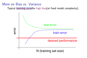
Experiencing high bias:

Low training set size: causes $J_{train}(\Theta )$ to be low and $J_{CV}(\Theta )$ to be high.

Large training set size: causes both $J_{train}(\Theta )$ and $J_{CV}(\Theta )$ to be high with $J_{train}(\Theta )$ ≈ $J_{CV}(\Theta$.

If a learning algorithm is suffering from high bias, getting more training data will not (by itself) help much.

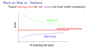
Experiencing high variance:

Low training set size: $J_{train}(\Theta )$ train will be low and $J_{CV}(\Theta )$ will be high.

Large training set size: $J_{train}(\Theta )$ increases with training set size and $J_{CV}(\Theta )$ continues to decrease without leveling off. Also, $J_{train}(\Theta )$ < $J_{CV}(\Theta )$ but the difference between them remains significant.

If a learning algorithm is suffering from high variance, getting more training data is likely to help.

---

在非常少的数据点(比如1、2或3)上训练一个算法很容易就不会有任何错误，因为我们总是可以找到一条二次曲线，它正好接触到这些数据点。 因此：

• 随着训练集的增大，二次函数的误差也会增大。

• 误差值在达到一定的m或训练集大小后会趋于稳定。The error value will

遇到高偏差：

小规模训练集： 会导致 $J_{train}(\Theta )$ 低而 $J_{CV}(\Theta )$ 大。

大规模训练集： 会导致 $J_{train}(\Theta )$ 和 $J_{CV}(\Theta )$ 都很大 ，同时$J_{train}(\Theta )$ ≈ $J_{CV}(\Theta )$.

如果一个学习算法存在高偏差，那么获得更多的训练数据对解决高偏差问题并没有多大帮助。

遇到高方差：

小规模训练集： $J_{train}(\Theta )$ 会很小而 $J_{CV}(\Theta )$ 会很大

大规模训练集： $J_{train}(\Theta )$ 随训练集大小的增加而增加，$J_{CV}(\Theta )$继续减少而不趋于平稳。 另外，$J_{train}(\Theta )$ < $J_{CV}(\Theta )$，但两者之间仍然有显著的差异。

如果一个学习算法有高方差，获得更多的训练数据可能会有帮助。

（4）Deciding What to Do Next Revisited

The relationship between them：

• High bias —— underfitting
• High variance —— overfitting

Our decision process can be broken down as follows:

1. Getting more training examples: Fixes high variance

2. Trying smaller sets of features: Fixes high variance

3. Adding features: Fixes high bias

4. Adding polynomial features: Fixes high bias

5. Decreasing λ（It’s like reducing the penalty factor）: Fixes high bias

6. Increasing λ（It’s like increasing the penalty factor）: Fixes high variance.

Diagnosing Neural Networks

• A neural network with fewer parameters is prone to underfitting. It is also computationally cheaper.

• A large neural network with more parameters is prone to overfitting. It is also computationally expensive. In this case you can use regularization (increase λ) to address the overfitting.

Using a single hidden layer is a good starting default. You can train your neural network on a number of hidden layers using your cross validation set. You can then select the one that performs best.

Model Complexity Effects:

• Lower-order polynomials (low model complexity) have high bias and low variance. In this case, the model fits poorly consistently.

• Higher-order polynomials (high model complexity) fit the training data extremely well and the test data extremely poorly. These have low bias on the training data, but very high variance.

• In reality, we would want to choose a model somewhere in between, that can generalize well but also fits the data reasonably well.

---

两者之间的关系：

• 高偏差 —— 欠拟合
• 高方差 —— 过拟合

我们的决策过程可以分解如下:

1. 获得更多的训练样本： 解决高方差

2. 使用更少的特征集： 解决高方差

3. 增加特征： 解决高偏差

4. 增加多项式特征: 解决高偏差

5. 减小 λ（相当于是减小惩罚因子）: 解决高偏差

6. 增大 λ（相当于是增大惩罚因子）: 解决高方差.

诊断神经网络

• 参数较少的神经网络容易出现欠拟合。 它的计算成本也更低。.

• 具有更多参数的大型神经网络容易出现过拟合。 它的计算成本也很高。 在这种情况下，你可以使用正则化（增加λ）来处理过拟合。

使用单个隐藏层是一个很好的初始默认值。你可以使用交叉验证集在有多个隐藏层的模型上训练神经网络。 然后，你可以选择性能最好的一个。

模型复杂性的影响：

• 低阶多项式（模型复杂度低）具有较高的偏差和较低的方差。在这种情况下，模型的一致性很差。

• 高阶多项式（模型复杂度高）对训练数据的拟合非常好，对测试数据的拟合非常差。这些对训练数据的偏差很低，但方差很高。

• 在现实中，我们希望选择一个介于两者之间的模型，既有很好的泛化能力，又能很好地拟合数据。

Machine Learning System Design

1. Building a Spam Classifier（构建垃圾邮件分类器）

Error Analysis

The recommended approach to solving machine learning problems is to:

• Start with a simple algorithm, implement it quickly, and test it early on your cross validation data.
• Plot learning curves to decide if more data, more features, etc. are likely to help.
• Manually examine the errors on examples in the cross validation set and try to spot a trend where most of the errors were made.
  

---

解决机器学习问题的推荐方法是：

• 从一个简单的算法开始，快速实现它，并在交叉验证数据中尽早测试它。
• 绘制学习曲线来决定更多的数据、更多的特征等是否有帮助。
• 手动检查交叉验证集中的样例中的错误，并尝试找出大多数错误产生的趋势。
  

2. Handling Skewed Data（处理数据倾斜问题）

（1）Error metrics for skewed classes（针对数据倾斜的混淆矩阵）

在收集到的数据集中，某种情况（例如y=0）占据总样本的比例过于大（例如95%），这种情况就叫做数据倾斜。此时，如果还用之前课程中的分类误差或者分类准确率来评判模型的好坏就很不合适。因此，提出了Error metrics（混淆矩阵也称误差矩阵）这种方式。

混淆矩阵是分类是一种衡量指标的格式，根据此格式可以得到Precision（查准率）Recall（召回率）。

矩阵中分为：真正例（true positive）、假正例（false positive）、真反例（true negative）、假反例（flase negative），用TP、FP、TN、FN来表示。
显然，样例总数 = TP+FP+TN+FN

$查准率（Precision）=\frac{TP}{TP+FP}$

查准率主要是针对预测样本来讨论，在预测的正例结果中有多少真正的正例被预测出来。（预测结果精确性的能力）

$召回率（Recall）=\frac{TP}{TP+FN}$

召回率主要是针对实际样本来讨论，在实际的正例样本中有多少正例被正确的预测出来。（找回正确结果个数的能力）

注：
在规定y = 1和y = 0时，通常选择样本中出现较少的情况规定为y = 1，即让稀有的为正例，较多的为反例。

（2）Trading Off Precision and Recall（权衡查准率和召回率）

阈值（threshold value）的大小将会影响着侧重于查准率（Precision）还是召回率（Recall）。当阈值偏大时（例如0.9），就会对预测出是否是正例（y=1）更加严格，则查准率就会上升，而召回率则会下降。当阈值偏小时（例如0.3），会就对预测出是否是正例（y=1）相对宽松一些，则召回率机就会上升，而查准率则会下降。查准率和召回率是一对矛盾的度量。一个高了，另一个就会变低。

很多情形下，我们可以根据学习器的预测结果（即学习器预测为正例的概率）对样本进行排序，排在前面的是学习器认为“最可能”是正例的样本，最后的则是学习器认为最不可能是正例的样本。按照此顺序逐个把样本作为正例进行预测，则每次都可计算出当前的查全率和查准率。以查准率为纵轴、查全率为横轴作图，得到查准率-查全率曲线，简称“P-R曲线”,给出一个示意图如下：

P-R图直观地显示出学习器在样本总体上的查全率、查准率。在进行学习器性能比较时，若一个学习器的P-R曲线完全包住另一个学习器的曲线，则断言前者的性能优于后者。在上图中，学习器A的性能优于学习器C。但是当两个学习器的P-R曲线发生交叉时，例如图中的A与B，则难以判断两个学习器的好坏。若要将AB两个学习器比较高低，一种合理的判据是比较P-R曲线下的面积大小，它在一定程度上表征了学习器在查准率和查全率上取得相对“双高”的比例。但是这个值不太容易估计，因此人们设计了一些综合考虑查全率与查准率的性能度量。

“平衡点（BEP）”就是一种度量方式，它是“查准率=查全率”时的取值。在上图中，基于BEP的比较，可认为学习器A优于B。

BEP过于简单，更常用的是F1度量：
$$F1=\frac{2PR}{P+R}=\frac{2TP}{样例总数+TP-TN}$$
其中F1是基于查准率与查全率的调和平均（harmonic mean）定义的：
$$\frac{1}{F1}=\frac{1}{2}\cdot (\frac{1}{P}+\frac{1}{R})$$

3. Using Large Data Sets（使用大规模数据集）

使用有许多参数的学习算法，可以让模型有低偏差，$J_{train}(\Theta )$ 将会很小；
使用有更大规模的数据集，可以让模型有低方差，$J_{train}(\Theta )\approx J_{test}(\Theta )$ 且 $J_{test}(\Theta )$ 将会很小。

如果，只增加参数，而数据集太小，将会引起高方差，即过拟合现象。如果仅增大数据集规模收集更多数据，而不增加特征数量，那么对已有高偏差的模型（欠拟合），可能没有太多帮助。

因此，收集更多的数据的同时增加更多参数，可以让模型既有低偏差，又有低方差。

Exercise 5：正则化线性回归与偏差和方差的对比

【吴恩达机器学习】Week6 编程作业ex5——正则化线性回归与偏差和方差的对比