SuperSeries 超gse号geo下载并处理表达矩阵duqiang同一个gse数据集里存在不同的测序平台产生的数据 生信技能树——GEO芯片数据的合并 如何去除批次效应 rnaseq去除批次效应

GSE70867
This SuperSeries is composed of the following SubSeries: Less…

GSE70864 BAL cell gene expression is predictive of Mortality in Idiopathic Pulmonary Fibrosis and enriched for Genes of Airway Basal Cells (I)

GSE70866 BAL cell gene expression is predictiveof Mortality in Idiopathic Pulmonary Fibrosis and enriched for Genesof Airway Basal Cells (II)

GSE73394 BAL cell gene expression is predictive of Mortality in Idiopathic Pulmonary Fibrosis and enrichedfor Genes of Airway Basal Cells (III)

GSE73395 BAL cell geneexpression is predictive of Mortality in Idiopathic Pulmonary Fibrosis and enriched for Genes of Airway Basal Cells (IV)

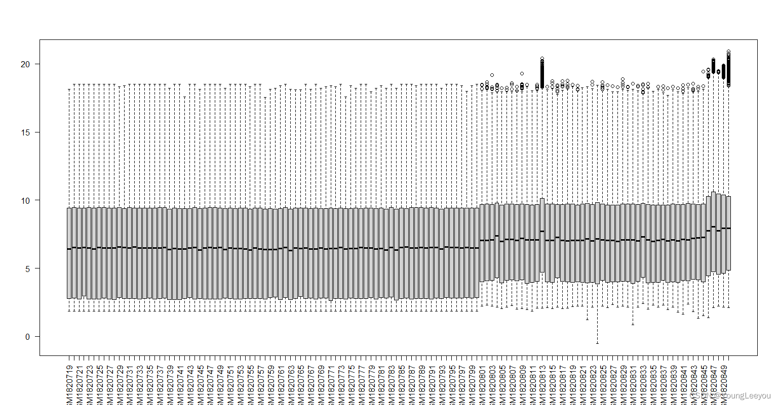
head(exprs(gset[[2]])) #gseGSE70867    

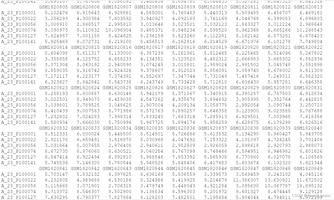
我发现超gse号里面的矩阵表达值和其子集的表达值一致，怎么会这样呢 超gse号里面多了其他样本啊 怎么最后归一化的矩阵表达量没有变呢 难道这是原始数据rawdata 不是normalized之后的数据？

**

同一个gse数据集里存在不同的测序平台产生的数据

**

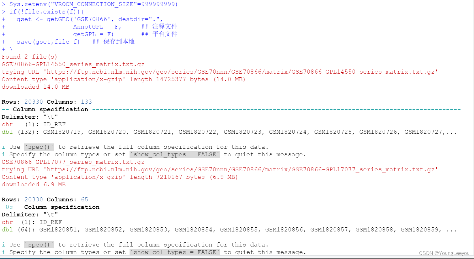
> getwd()
[1] "G:/r/duqiang_IPF/GSE70866—true—_BAL_IPF_donors_RNA-seq"
> class(gset)  #查看数据类型
[1] "list"
> length(gset)  #
[1] 2
> class(gset[[1]])
[1] "ExpressionSet"
attr(,"package")
[1] "Biobase"
> gset
$`GSE70866-GPL14550_series_matrix.txt.gz`
ExpressionSet (storageMode: lockedEnvironment)
assayData: 20330 features, 132 samples 
  element names: exprs 
protocolData: none
phenoData
  sampleNames: GSM1820719 GSM1820720 ... GSM1820850 (132 total)
  varLabels: title geo_accession ... time to death (days):ch1 (46 total)
  varMetadata: labelDescription
featureData: none
experimentData: use 'experimentData(object)'
  pubMedIds: 30141961 
Annotation: GPL14550 

$`GSE70866-GPL17077_series_matrix.txt.gz`
ExpressionSet (storageMode: lockedEnvironment)
assayData: 20330 features, 64 samples 
  element names: exprs 
protocolData: none
phenoData
  sampleNames: GSM1820851 GSM1820852 ... GSM1820914 (64 total)
  varLabels: title geo_accession ... time to death (days):ch1 (46 total)
  varMetadata: labelDescription
featureData: none
experimentData: use 'experimentData(object)'
  pubMedIds: 30141961 
Annotation: GPL17077 

> gset[[1]]@annotation # 平台信息——提取芯片平台编号
[1] "GPL14550"

$GSE70866-GPL17077_series_matrix.txt.gz :

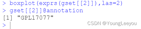
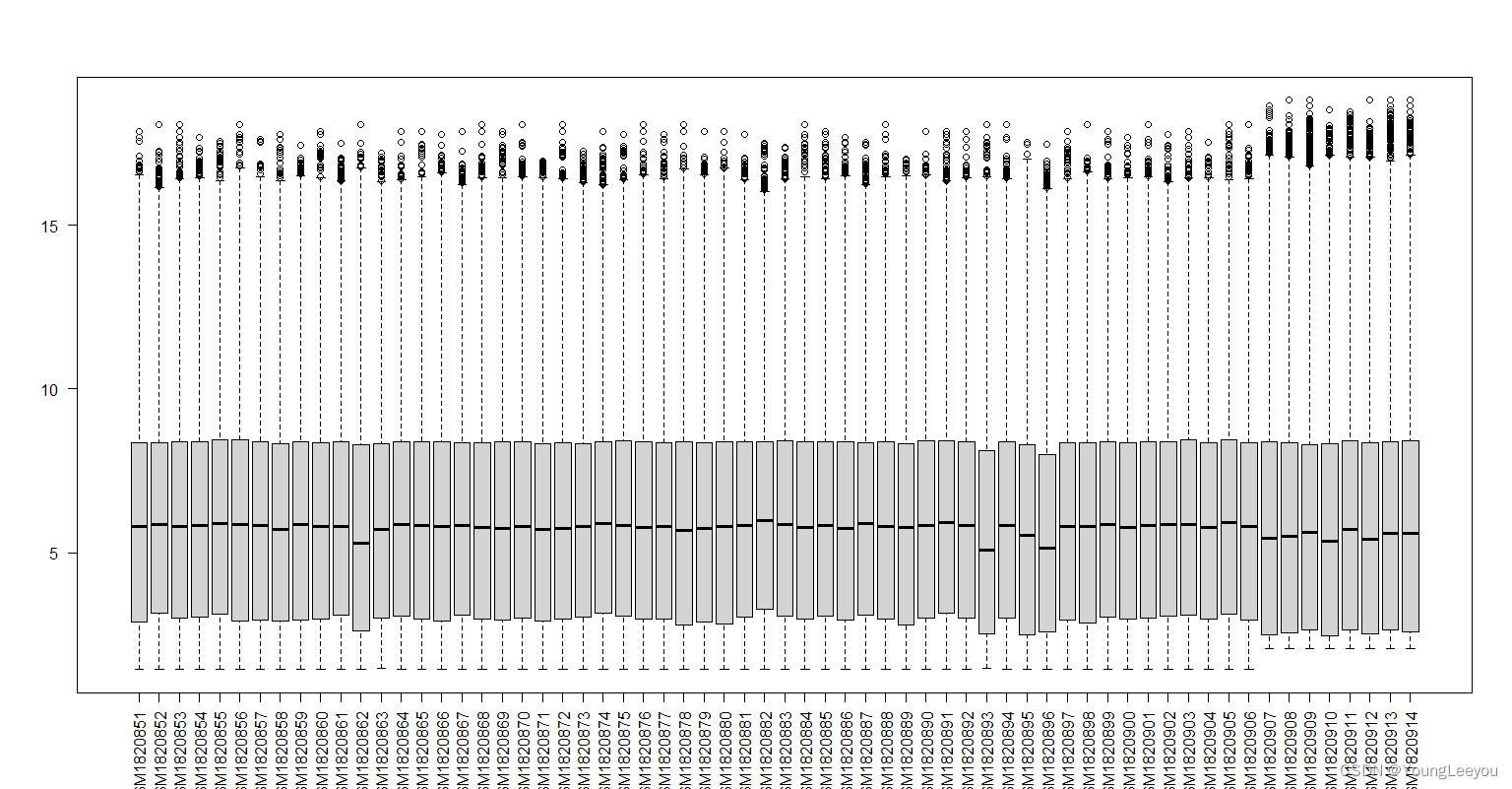
colnames(exprs(gset[[2]]))
[1] “GSM1820851” “GSM1820852” “GSM1820853” “GSM1820854” “GSM1820855”
[6] “GSM1820856” “GSM1820857” “GSM1820858” “GSM1820859” “GSM1820860”
[11] “GSM1820861” “GSM1820862” “GSM1820863” “GSM1820864” “GSM1820865”
[16] “GSM1820866” “GSM1820867” “GSM1820868” “GSM1820869” “GSM1820870”
[21] “GSM1820871” “GSM1820872” “GSM1820873” “GSM1820874” “GSM1820875”
[26] “GSM1820876” “GSM1820877” “GSM1820878” “GSM1820879” “GSM1820880”
[31] “GSM1820881” “GSM1820882” “GSM1820883” “GSM1820884” “GSM1820885”
[36] “GSM1820886” “GSM1820887” “GSM1820888” “GSM1820889” “GSM1820890”
[41] “GSM1820891” “GSM1820892” “GSM1820893” “GSM1820894” “GSM1820895”
[46] “GSM1820896” “GSM1820897” “GSM1820898” “GSM1820899” “GSM1820900”
[51] “GSM1820901” “GSM1820902” “GSM1820903” “GSM1820904” “GSM1820905”
[56] “GSM1820906” “GSM1820907” “GSM1820908” “GSM1820909” “GSM1820910”
[61] “GSM1820911” “GSM1820912” “GSM1820913” “GSM1820914”

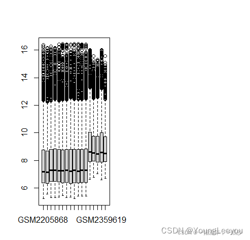
boxplot(exprs(gset[[2]]),las=2)

如何去除批次效应

GSE83521和GSE89143数据合并
1.下载数据
rm(list = ls())
library(GEOquery)
library(stringr)
gse = "GSE83521"
eSet1 <- getGEO("GSE83521", 
                destdir = '.', 
                getGPL = F)
eSet2 <- getGEO("GSE89143", 
                destdir = '.', 
                getGPL = F)
#(1)提取表达矩阵exp
exp1 <- exprs(eSet1[[1]])
exp1[1:4,1:4]
exp2 <- exprs(eSet2[[1]])
exp2[1:4,1:4]
exp2 = log2(exp2+1)
table(rownames(exp1) %in% rownames(exp2))
length(intersect(rownames(exp1),rownames(exp2)))
exp1 <- exp1[intersect(rownames(exp1),rownames(exp2)),]
exp2 <- exp2[intersect(rownames(exp1),rownames(exp2)),]
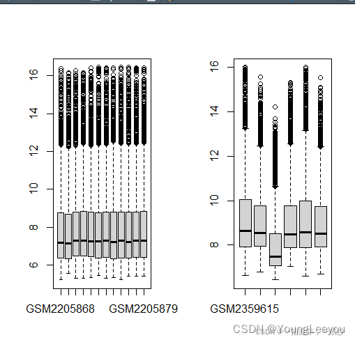
boxplot(exp1)
boxplot(exp2)

#(2)提取临床信息
pd1 <- pData(eSet1[[1]])
pd2 <- pData(eSet2[[1]])
if(!identical(rownames(pd1),colnames(exp1))) exp1 = exp1[,match(rownames(pd1),colnames(exp1))]
if(!identical(rownames(pd2),colnames(exp2))) exp2 = exp2[,match(rownames(pd2),colnames(exp2))]

#(3)提取芯片平台编号
gpl <- eSet2[[1]]@annotation

#(4)合并表达矩阵
# exp2的第三个样本有些异常，可以去掉或者用normalizeBetweenArrays标准化，把它拉回正常水平。

exp2 = exp2[,-3]

exp = cbind(exp1,exp2)
boxplot(exp)
Group1 = ifelse(str_detect(pd1$title,"Tumour"),"Tumour","Normal")
Group2 = ifelse(str_detect(pd2$source_name_ch1,"Paracancerous"),"Normal","Tumour")[-3]

Group = c(Group1,Group2)
table(Group)
Group = factor(Group,levels = c("Normal","Tumour"))
save(gse,Group,exp,gpl,file = "exp.Rdata")

两个数据集样本的情况

合并之后的数据

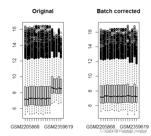
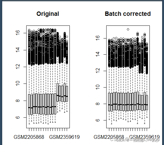
2.针对不同数据集数据的差异，需要处理批次效应
2.1 使用limma包里的removeBatchEffect()函数
rm(list = ls())
load("exp.Rdata")
#处理批次效应
library(limma)
#?removeBatchEffect()
batch <- c(rep("A",12),rep("B",5))
exp2 <- removeBatchEffect(exp, batch)
par(mfrow=c(1,2))  # 展示的图片为一行两列
boxplot(as.data.frame(exp),main="Original")
boxplot(as.data.frame(exp2),main="Batch corrected")

2.2 使用sva包中的combat() 函数
rm(list = ls())
load("exp.Rdata")
#处理批次效应(combat)
library(sva)
#?ComBat

batch <- c(rep("A",12),rep("B",5))
mod = model.matrix(~Group)
exp2 = ComBat(dat=exp, batch=batch, 
              mod=mod, par.prior=TRUE, ref.batch="A")
par(mfrow=c(1,2))
boxplot(as.data.frame(exp),main="Original")
boxplot(as.data.frame(exp2),main="Batch corrected")