
【pandas】用户手册:10分钟熟悉pandas(下)
数据分组
Splitting: 利用某些条件将数据进行分组Applying: 函数应用于每个单独的分组Combining: 合并最终的结果
df = pd.DataFrame(
    {
        "A": ["foo", "bar", "foo", "bar", "foo", "bar", "foo", "foo"],
        "B": ["one", "one", "two", "three", "two", "two", "one", "three"],
        "C": np.random.randn(8),
        "D": np.random.randn(8),
    }
)
df
     A      B         C         D
0  foo    one -0.738005 -2.019732
1  bar    one  0.887627  0.015670
2  foo    two -0.108933 -0.077614
3  bar  three  0.076641  1.675694
4  foo    two -0.787585  0.466678
5  bar    two  0.193921 -0.345819
6  foo    one  0.846988 -1.513333
7  foo  three  1.110915  0.189766
df.groupby("A")[["C", "D"]].sum()
            C         D
A
bar  1.158189  1.345545
foo  0.323379 -2.954235
分组并应用
sum()对他们进行求和汇总
df.groupby(["A", "B"]).sum()
                  C         D
A   B
bar one    0.887627  0.015670
    three  0.076641  1.675694
    two    0.193921 -0.345819
foo one    0.108983 -3.533064
    three  1.110915  0.189766
    two   -0.896518  0.389064
先对
A分组,后对B分组
df.groupby(["B", "A"]).sum()
                  C         D
B     A
one   bar  0.887627  0.015670
      foo  0.108983 -3.533064
three bar  0.076641  1.675694
      foo  1.110915  0.189766
two   bar  0.193921 -0.345819
      foo -0.896518  0.389064
先对
B分组,后对A分组
注意:对多个列进行操作,用
[["C", "D"]]
对一个列进行操作,可以用["C"], 当然也可以用[["C"]]
数据表格形状改变
Stack
tuples = list(
    zip(
        ["bar", "bar", "baz", "baz", "foo", "foo", "qux", "qux"],
        ["one", "two", "one", "two", "one", "two", "one", "two"],
    )
)
# tuples
# 多索引值
index = pd.MultiIndex.from_tuples(tuples, names=["first", "second"])
df = pd.DataFrame(np.random.randn(8, 3), columns=["C1", "C2", "C3"], index=index)
df2 = df[:5]
df2
                    C1        C2        C3
first second
bar   one    -1.347431  0.153681 -1.006217
      two    -0.741849 -0.117988 -0.593601
baz   one     0.394623 -0.360702  0.062728
      two    -0.477569 -1.504717  0.124419
foo   one     0.340487 -1.045430 -0.623986
stacked = df2.stack()
stacked
first  second
bar    one     C1   -1.347431
               C2    0.153681
               C3   -1.006217
       two     C1   -0.741849
               C2   -0.117988
               C3   -0.593601
baz    one     C1    0.394623
               C2   -0.360702
               C3    0.062728
       two     C1   -0.477569
               C2   -1.504717
               C3    0.124419
foo    one     C1    0.340487
               C2   -1.045430
               C3   -0.623986
dtype: float64
stack将数据压缩成一个列
上面例子中df2的shape为(5,3)
stacked的shape为(15, )
Pivot
创建一个电子表格风格的数据透视表作为数据框架。
函数原型:pandas.pivot_table(data, values=None, index=None, columns=None, aggfunc='mean', fill_value=None, margins=False, dropna=True, margins_name='All', observed=False, sort=True)
df = pd.DataFrame(
    {
        "C1": ["one", "one", "two", "three"] * 3,
        "C2": ["A", "B", "C"] * 4,
        "C3": ["foo", "foo", "foo", "bar", "bar", "bar"] * 2,
        "C4": np.random.randn(12),
        "C5": np.random.randn(12),
    }
)
df
       C1 C2   C3        C4        C5
0     one  A  foo -0.111176 -0.049645
1     one  B  foo -0.483144 -2.182207
2     two  C  foo  0.841522 -0.669410
3   three  A  bar  1.074447 -1.335228
4     one  B  bar -1.949381  0.594608
5     one  C  bar -1.544474 -0.873641
6     two  A  foo -0.837036 -1.054699
7   three  B  foo  0.537476 -0.359334
8     one  C  foo  0.169522 -1.594076
9     one  A  bar -0.595527  0.225416
10    two  B  bar -0.443136 -1.495795
11  three  C  bar -0.081103  1.551327
取
C1列的值作为新的label
取C2,C3列的值作为索引
取C5列的值作为表里的值, 无值则补NaN
pd.pivot_table(df, values="C5", index=["C2", "C3"], columns=["C1"])
C1           one     three       two
C2 C3
A  bar  0.225416 -1.335228       NaN
   foo -0.049645       NaN -1.054699
B  bar  0.594608       NaN -1.495795
   foo -2.182207 -0.359334       NaN
C  bar -0.873641  1.551327       NaN
   foo -1.594076       NaN -0.669410
时间序列
pandas 具有简单、强大、高效的功能,可以在变频过程中进行重采样操作(如将秒级数据转换为5分钟级数据)。这在(但不限于)金融应用程序中非常常见。请参阅时间序列部分。
rng = pd.date_range("1/1/2023", periods=100, freq="S")
ts = pd.Series(np.random.randint(0, 500, len(rng)), index=rng)
ts
2023-01-01 00:00:00    194
2023-01-01 00:00:01    306
2023-01-01 00:00:02     54
2023-01-01 00:00:03    198
2023-01-01 00:00:04    368
                      ...
2023-01-01 00:01:35    431
2023-01-01 00:01:36    276
2023-01-01 00:01:37    286
2023-01-01 00:01:38    223
2023-01-01 00:01:39    217
Freq: S, Length: 100, dtype: int32
ts.resample("5Min").sum()
2023-01-01    25350
Freq: 5T, dtype: int32
Series.tz_localize() localizes a time series to a time zone:
将时间序列化为本地化一个时区
rng = pd.date_range("1/6/2023 00:00", periods=5, freq="D")
ts = pd.Series(np.random.randn(len(rng)), rng)
ts_utc = ts.tz_localize('UTC')
ts_utc
2023-01-06 00:00:00+00:00    0.418221
2023-01-07 00:00:00+00:00   -1.714893
2023-01-08 00:00:00+00:00   -0.464742
2023-01-09 00:00:00+00:00    0.005428
2023-01-10 00:00:00+00:00    0.209386
Freq: D, dtype: float64
将一个时区转到另外一个时区
ts_utc.tz_convert("US/Eastern")
2023-01-05 19:00:00-05:00    0.418221
2023-01-06 19:00:00-05:00   -1.714893
2023-01-07 19:00:00-05:00   -0.464742
2023-01-08 19:00:00-05:00    0.005428
2023-01-09 19:00:00-05:00    0.209386
Freq: D, dtype: float64
数据分类
df["raw_grade"].astype("category")将raw_grade类型换成了类别。
df = pd.DataFrame(
    {"id": [1, 2, 3, 4, 5, 6], "raw_grade": ["a", "b", "b", "a", "a", "e"]}
)
df["grade"] = df["raw_grade"].astype("category")
df["grade"]
0    a
1    b
2    b
3    a
4    a
5    e
Name: grade, dtype: category
Categories (3, object): ['a', 'b', 'e']
rename_categories将类别名称重命名。
new_categories = ["very good", "good", "very bad"]
df["grade"] = df["grade"].cat.rename_categories(new_categories)
df["grade"]
0    very good
1         good
2         good
3    very good
4    very good
5     very bad
Name: grade, dtype: category
Categories (3, object): ['very good', 'good', 'very bad']
增加新的类别
df["grade"] = df["grade"].c> `df["raw_grade"].astype("category")` 将`raw_grade`类型换成了类别。at.set_categories(
    ["very bad", "bad", "medium", "good", "very good"]
)
df["grade"]
0    very good
1         good
2         good
3    very good
4    very good
5     very bad
Name: grade, dtype: category
Categories (5, object): ['very bad', 'bad', 'medium', 'good', 'very good']
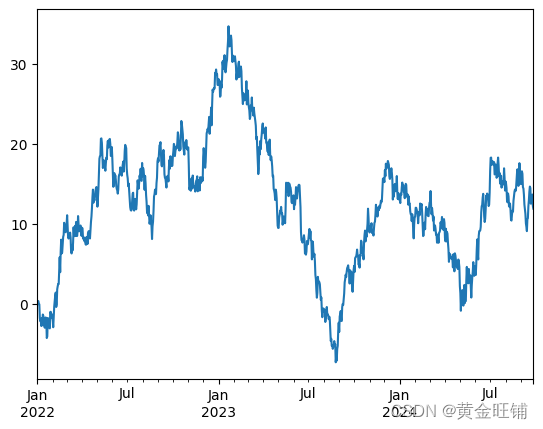
显示数据
import matplotlib.pyplot as plt
plt.close("all")
ts = pd.Series(np.random.randn(1000), index=pd.date_range("1/1/2022", periods=1000))
ts = ts.cumsum()
ts.plot()
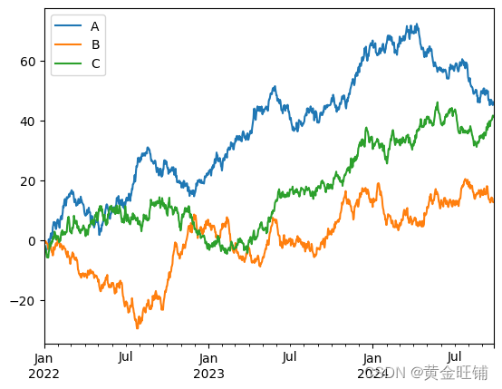
df = pd.DataFrame(np.random.randn(1000, 3), index=ts.index, columns=['A', 'B', 'C'])
df = df.cumsum()
plt.figure()
df.plot()
plt.legend(loc='best')
数据导入导出
CSV
df.to_csv("foo.csv")
pd.read_csv("foo.csv")
     Unnamed: 0          A          B          C
0    2022-01-01  -2.112172  -0.161145  -1.891843
1    2022-01-02  -1.787807  -0.469220  -1.592460
2    2022-01-03  -2.366840  -0.465609  -3.204489
3    2022-01-04  -2.913202  -0.220295  -3.415782
4    2022-01-05  -3.819952  -0.831654  -3.465468
..          ...        ...        ...        ...
995  2024-09-22  45.661361  13.760668  40.401864
996  2024-09-23  45.608082  14.161003  41.035935
997  2024-09-24  45.256665  12.934910  41.751221
998  2024-09-25  46.313781  12.783737  41.720967
999  2024-09-26  46.183519  12.790855  41.323802

[1000 rows x 4 columns]
HDF5
df.to_hdf("foo.h5", "df")
pd.read_hdf("foo.h5", "df")
这中间有可能会报错:
File d:\Anaconda3\envs\pytorch\lib\site-packages\pandas\compat\_optional.py:141, in import_optional_dependency(name, extra, errors, min_version)
    140 try:
--> 141     module = importlib.import_module(name)
    142 except ImportError:

File d:\Anaconda3\envs\pytorch\lib\importlib\__init__.py:127, in import_module(name, package)
    126         level += 1
--> 127 return _bootstrap._gcd_import(name[level:], package, level)

File <frozen importlib._bootstrap>:1014, in _gcd_import(name, package, level)

File <frozen importlib._bootstrap>:991, in _find_and_load(name, import_)

File <frozen importlib._bootstrap>:973, in _find_and_load_unlocked(name, import_)

ModuleNotFoundError: No module named 'tables'

During handling of the above exception, another exception occurred:

ImportError                               Traceback (most recent call last)
Cell In [90], line 1
----> 1 df.to_hdf("foo.h5", "df")
...
--> 144         raise ImportError(msg)
    145     else:
    146         return None

ImportError: Missing optional dependency 'pytables'.  Use pip or conda to install pytables.
提示用
pip install pytables但还是会报错,最后改用pip install tables解决问题;
`ERROR: Could not find a version that satisfies the requirement pytables (from versions: none)
ERROR: No matching distribution found for pytables
                    A          B          C
2022-01-01  -2.112172  -0.161145  -1.891843
2022-01-02  -1.787807  -0.469220  -1.592460
2022-01-03  -2.366840  -0.465609  -3.204489
2022-01-04  -2.913202  -0.220295  -3.415782
2022-01-05  -3.819952  -0.831654  -3.465468
...               ...        ...        ...
2024-09-22  45.661361  13.760668  40.401864
2024-09-23  45.608082  14.161003  41.035935
2024-09-24  45.256665  12.934910  41.751221
2024-09-25  46.313781  12.783737  41.720967
2024-09-26  46.183519  12.790855  41.323802

[1000 rows x 3 columns]
excel
ModuleNotFoundError: No module named 'openpyxl'
# pip install openpyxl
df.to_excel("foo.xlsx", sheet_name="Sheet1")
pd.read_excel("foo.xlsx", "Sheet1", index_col=None, na_values=["NA"])
    Unnamed: 0          A          B          C
0   2022-01-01  -2.112172  -0.161145  -1.891843
1   2022-01-02  -1.787807  -0.469220  -1.592460
2   2022-01-03  -2.366840  -0.465609  -3.204489
3   2022-01-04  -2.913202  -0.220295  -3.415782
4   2022-01-05  -3.819952  -0.831654  -3.465468
..         ...        ...        ...        ...
995 2024-09-22  45.661361  13.760668  40.401864
996 2024-09-23  45.608082  14.161003  41.035935
997 2024-09-24  45.256665  12.934910  41.751221
998 2024-09-25  46.313781  12.783737  41.720967
999 2024-09-26  46.183519  12.790855  41.323802

[1000 rows x 4 columns]
【参考】
10 minutes to pandas — pandas 1.5.2 documentation (pydata.org)
相关文章
- Py之pandas:字典格式数据与dataframe格式数据相互转换并导出到csv
- 100天精通Python(数据分析篇)——第70天:Pandas常用排序、排名方法(sort_index、sort_values、rank)
- python pandas自定义函数之apply函数用法
- Pandas 横向合并DataFrame数据
- Python数据科学pandas终极指南【看这篇文章就够了】
- pandas入门10分钟——serries其实就是data frame的一列数据
- Pandas学习导图
- 数据分析工具Pandas基础 数据清洗--处理缺失数据、处理重复数据、替换数据处理
- 如何在 Pandas DataFrame 列中搜索值?
- pandas多键值merge