【信号处理】基于优化算法的 SAR 信号处理（Matlab代码实现）

💥💥💥💞💞💞欢迎来到本博客❤️❤️❤️💥💥💥

🏆博主优势：🌞🌞🌞博客内容尽量做到思维缜密，逻辑清晰，为了方便读者。
🚀支持：🎁🎁🎁如果觉得博主的文章还不错或者您用得到的话，可以关注一下博主，如果三连收藏支持就更好啦！这就是给予我最大的支持！

​

📋📋📋本文目录如下：⛳️⛳️⛳️

目录

1 概述

2 运行结果 

3 Matlab代码实现

1 概述

本文包括：

1. 提供的4种目标空气重建算法的分离和模块化：2D匹配滤波（波前重建），时域相关性（TDC），背投（BP）和范围堆叠（RS）。
2. 用现代渲染命令替换过时的图形命令，清楚地显示DSP操作对SAR信号的影响。
3. 删除笨拙的代码，对 （kx，ky） 域中分布不均匀的数据进行 2D 插值，并替换为更不繁琐、更优雅的现代 MatLab 命令。
4. 尽可能按照书籍符号和命名法为重要的SAR信号分配专有名称。此外，我还提供了所有这些SAR信号及其域的详细表格。
5. 添加了几个脚本，计算AM-PM和PM球面SAR信号的CTFT，既有数字形式，也有使用稳态相位近似（SPA）方法。
6. 几个小的代码改进。

2 运行结果 

这里仅展现部分运行结果：

​

​ ​ ​ ​ ​ 部分代码：

%% Fresnel Approximation of a PM Signal by a Chirp Signal

%% Workspace Initialization.
clc; clear; close all;

%% Radar System Parameters       
c  = 3e8;            % propagation speed
fc = 250e6;          % frequency
lambda = c/fc;       % Wavelength
k = 2*pi/lambda;     % Wavenumber
Xc = 2e3;            % Range distance to center of target area

%% Case 1: Broadside Target Area
L  = 300;             % synthetic aperture is 2*L
Y0 = 100;             % target area in cross-range is within [Yc-Y0,Yc+Y0]
Yc = 0;               % Cross-range distance to center of target area
du = 0.05;
u = -L:du:L;
xn = Xc;
yn = 50;

%% Signal Definitions - Fresnel Approximation 
% $$\exp[-j2k \sqrt{x_n^2 + (y_n - u)^2}] \approx \exp\Bigg[-j2kx_n -
% j\frac{k(y_n - u)^2}{X_c}\Bigg]$$

%%%%%%%%%%%%%%%%%%%%%%%%%%%%%%%%%%%%%%%%%%%%%%%%%%%%%%%%%%$%
%   Program to compare between the original PM signal and  %
%   Fresnel Approximation                                  %
%%%%%%%%%%%%%%%%%%%%%%%%%%%%%%%%%%%%%%%%%%%%%%%%%%%%%%%%%%$%

% Original Spherical PM Signal:
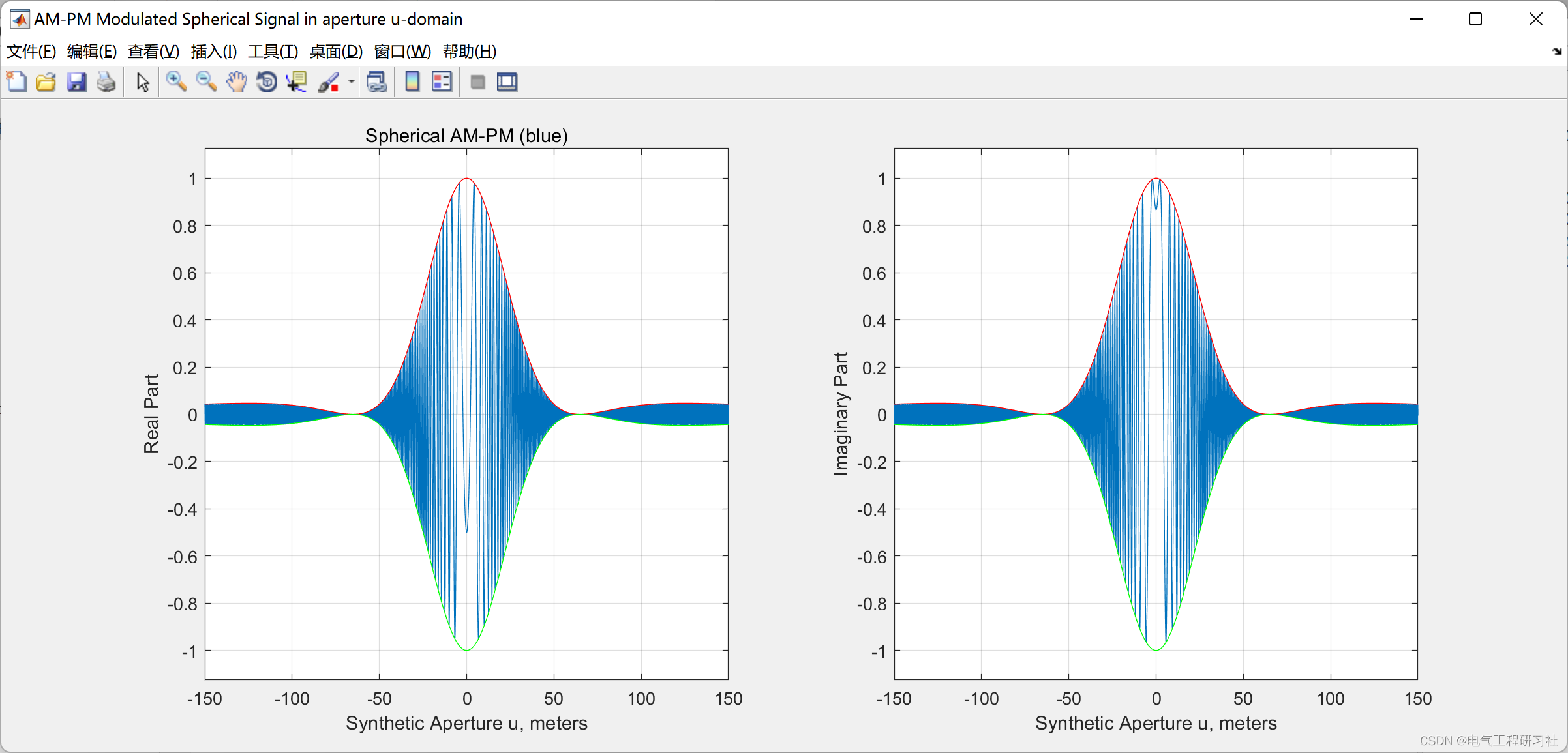
PM = exp(-1i*2*k*sqrt(xn^2+(yn-u).^2));

% Fresnel Chirp Approximation:
FA = exp(-1i*2*k*(xn+((yn-u).^2)/Xc/2));

%% Plot the Spherical PM and Chirp Approximation Signals.
h1 = figure('NumberTitle', 'off','Name','Comparison of PM and Fresnel Approximation', ...
            'Position', [100 0 1200 1000]);

subplot(2,2,1)
plot(u,real(PM))
title('Spherical PM (blue) - Fresnel Chirp Approx. (red)')
hold on;
plot(u,real(FA),'r.')
xlabel('Synthetic Aperture u, meters')
ylabel('Real Part')
axis([-250 250 1.25*min(real(PM)) 1.25*max(real(PM))]);
grid on;

subplot(2,2,2)
plot(u,real(PM) - real(FA),'g.')
xlabel('Synthetic Aperture u, meters')
ylabel('Real Part')
title('Real Part Approximation Error')
grid on;
axis([-250 250 1.25*min(real(PM)) 1.25*max(real(PM))]);
grid on;

subplot(2,2,3)
plot(u,imag(PM))
hold on;
plot(u,imag(FA),'r.')
title('Spherical PM (blue) - Fresnel Chirp Approx. (red)')
xlabel('Synthetic Aperture u, meters')
ylabel('Imaginary Part')
axis([-250 250 1.25*min(imag(FA)) 1.25*max(imag(FA))]);
grid on;

subplot(2,2,4)
plot(u,imag(PM) - imag(FA),'m.')
xlabel('Synthetic Aperture u, meters')
ylabel('Imaginary Part')
title('Imaginary Part Approximation Error')
grid on;
axis([-250 250 1.25*min(imag(FA)) 1.25*max(imag(FA))]);
grid on;

%% Phase Comparison
h2 = figure('NumberTitle', 'off','Name','Comparison of PM and Fresnel Approximation', ...
            'Position', [100 0 1200 500]);

subplot(1,2,1)
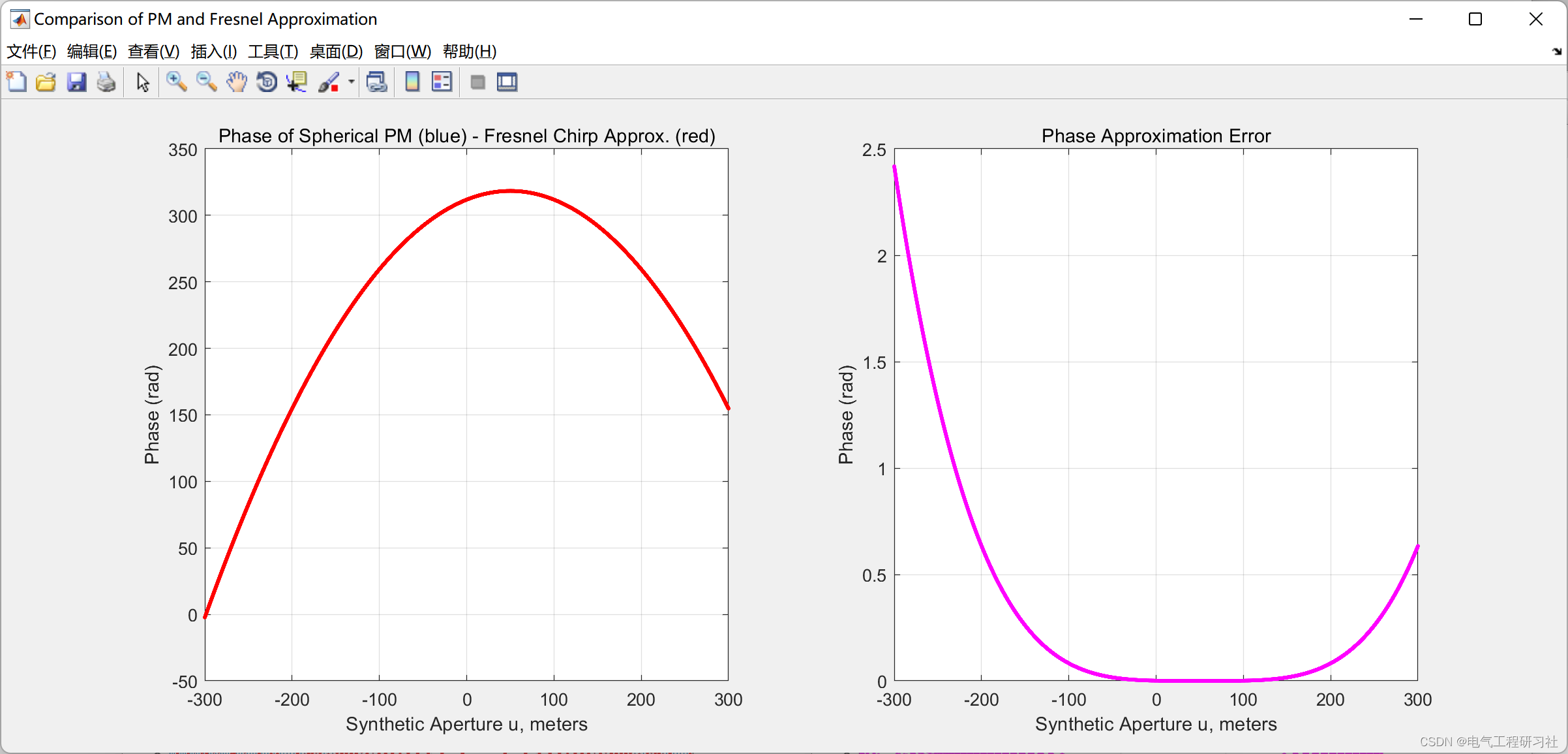
plot(u,unwrap(angle(PM)))
hold on;
plot(u,unwrap(angle(FA)),'r.')
title('Phase of Spherical PM (blue) - Fresnel Chirp Approx. (red)')
xlabel('Synthetic Aperture u, meters')
ylabel('Phase (rad)')
grid on;

subplot(1,2,2)
plot(u,unwrap(angle(PM)) - unwrap(angle(FA)),'m.')
xlabel('Synthetic Aperture u, meters')
ylabel('Phase (rad)')
title('Phase Approximation Error')
grid on;

3 Matlab代码实现