
【灵敏性】用于二维和三维声学设计灵敏度分析的奇异边界法(Matlab代码实现)
💥💥💞💞欢迎来到本博客❤️❤️💥💥
🏆博主优势:🌞🌞🌞博客内容尽量做到思维缜密,逻辑清晰,为了方便读者。
⛳️座右铭:行百里者,半于九十。
📋📋📋本文目录如下:🎁🎁🎁
目录

💥1 概述
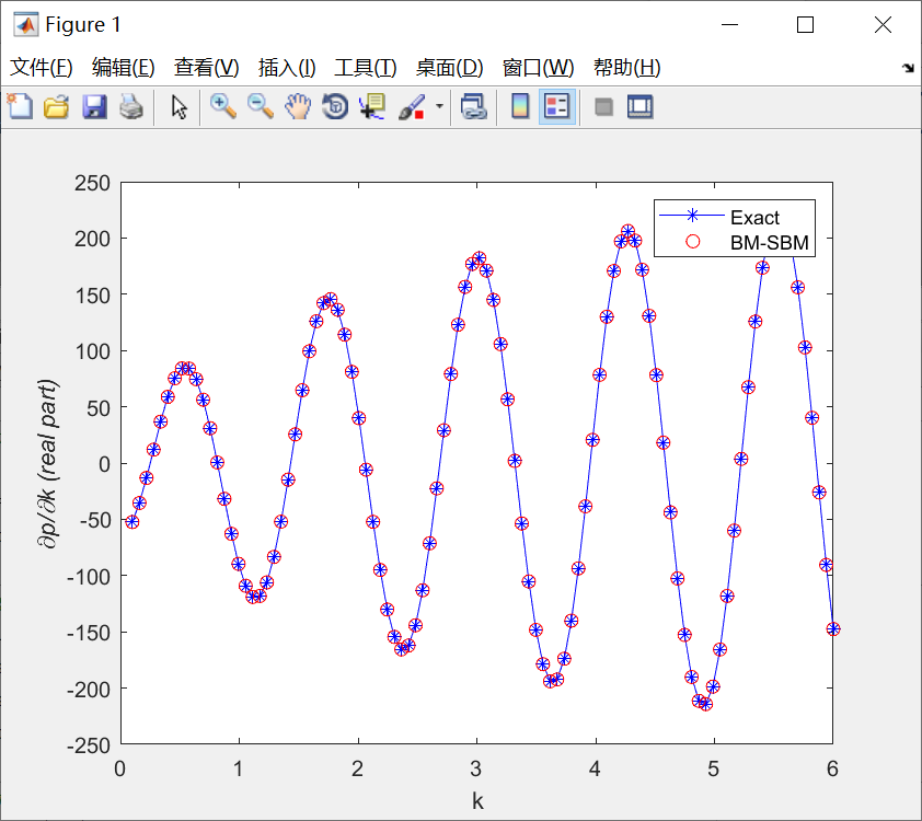
奇异边界法是一类半解析边界无网格配点技术,是用于计算科学与工程问题的新型数值算法之一。类似于边界元法,奇异边界法采用波传播方程的基本解作为插值基函数;不同之处在于,奇异边界法引入源点强度因子的概念来代替基本解的源点奇异性,避免处理边界元法中数学复杂的奇异与近奇异数值积分。奇异边界法的关键在于选取合适的计算方法确定源点强度因子。为提高声学灵敏度分析数值计算的速度和准确性,充分利用Burton-Miller公式和奇异边界法的优势,采用MATLAB软件对声学灵敏度分析进行程序设计与实现,生成基于MATLAB的Burton-Miller奇异边界法图形用户界面(graphical user interface, GUI)。使用该程序对典型声学灵敏度分析算例进行计算,结果表明该程序具有简洁易懂、操作方便、计算结果精确可靠等优点,是一种简洁、高效、实用的模拟工具。本文章将介绍使用该方法对二维和三维声学设计灵敏度进行分析。
📚2 运行结果
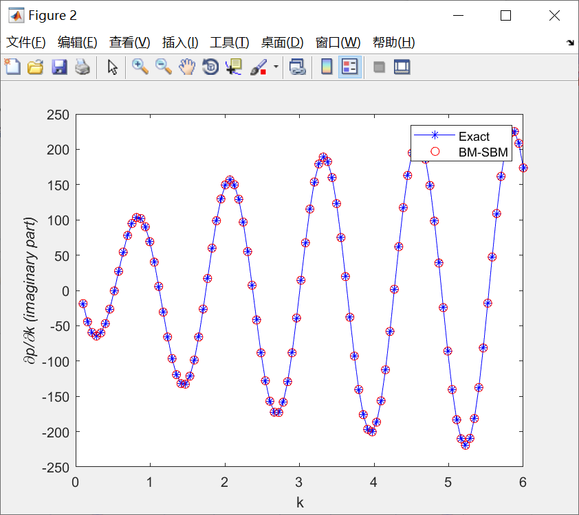
二维:
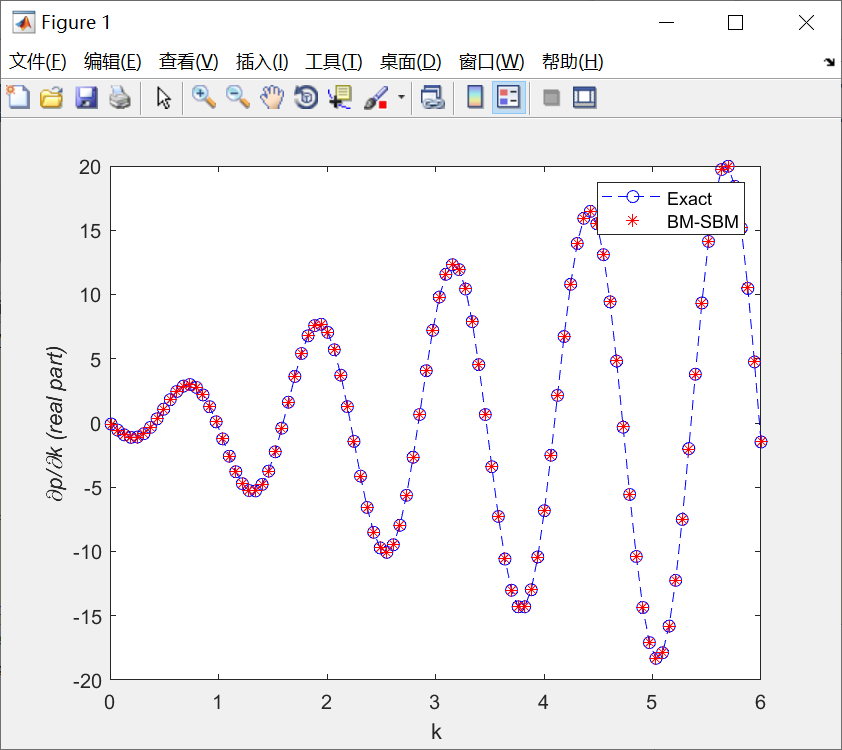
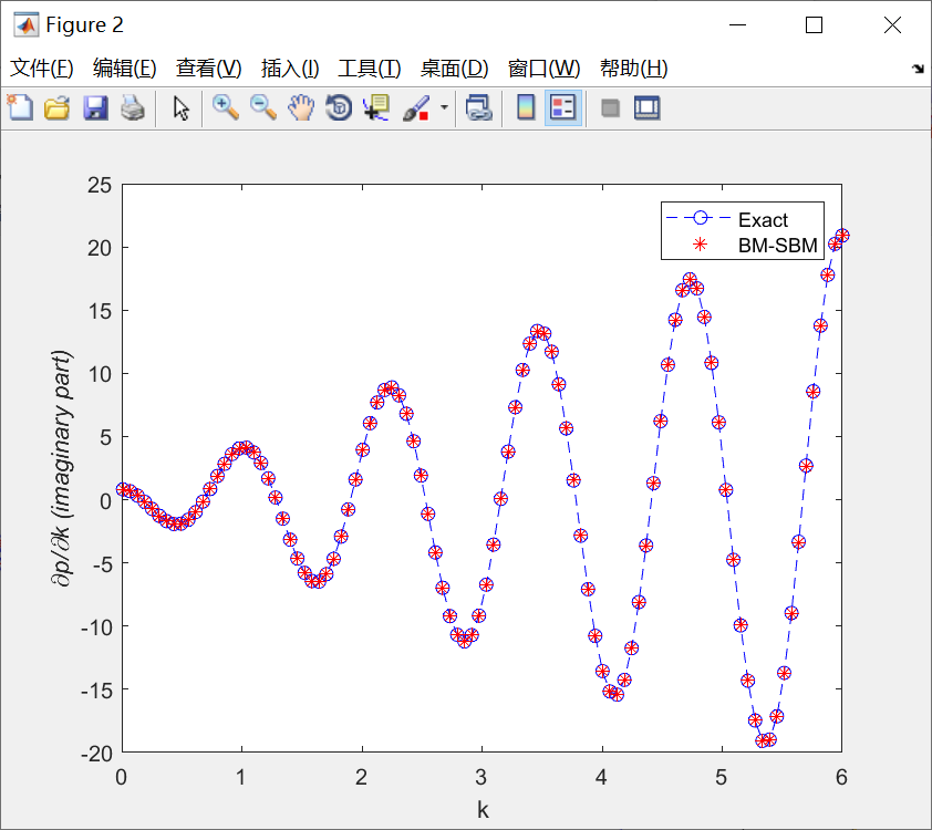
三维:
部分代码(三维主函数):
%=========================================================================
% Essay topic:
% Singular boundary method for 2D and 3D acoustic design
% sensitivity analysis
%
%
%=========================================================================
% benchmark example:
% 3D acoustic sensitivity analysis for
% Oscillating sphere
% ---Neumann boundary condition
% ---Acoustic sensitivity with respect
% to the wave number k
% %% Attention:
% The results of the paper are the results obtained by
% running the code in the software Matlab2019a.
% ---Computations are implemented on a laptop with
% an AMD Ryzen 7 4800H CPU at 2.90 GHz
% on a 64-bit Windows 10 with 16G RAM.
%
%=========================================================================
clear all;
clc;
format long
%% Parameter settings
t0 = clock; % Time Start
n = 100; % Total number of soource points
m = 100; % The number of equal parts for design variable
a = 0.1; % Radius of pulsating cylinder
SS = 4*pi*a^2;
Lj = SS/n; % The influence ranges of source point.
rho = 1.2; % the air density
c = 341; % The speed of sound in air
v0=1; % the radial velocity
k = linspace(0.01,6,m); % The value range of the wave number
dk = (k(end)-k(1))/(m-1);
xi = 5 ; yi = 0; zi = 0; % test point
i = sqrt(-1);
%% Analytical solution of the acoustic sensitivity with respect to the wave number
pt_exact = @(ro,k,a) i*rho*c*v0*a^2*exp(i*k.*(ro-a))./(ro.*(1-i*k*a).^2).*((1-i*k*a).^2+i*k*ro.*(1-i*k*a)+i*k*a);
%% Arrangement of Boundary Points
[nodes] = Creat_Sources(n);
xp = a.*nodes(:, 1);
yp = a.*nodes(:, 2);
zp = a.*nodes(:, 3);
n_x = -xp/a; n_y = -yp/a; n_z = -zp/a;
r=sqrt((xp-xp').^2+(yp-yp').^2+(zp-zp').^2);
%% Unknown coefficient solving process
alpha = zeros(n,m);
for j=1:m
lamda=i/(k(j)+1);
b = i*rho*k(j)*c*v0*ones(n,1) ; % boundary condition (Nuemann)
[~,F,~,H] = GFEH(k(j),r,xp,yp,zp,xp',yp',zp',n_x,n_y,n_z,n_x',n_y',n_z');
A=F+lamda*H;
[~,H0] = FH0(r,xp,yp,zp,xp',yp',zp',n_x,n_y,n_z,n_x',n_y',n_z');
[~,E0] = GE0(r,xp,yp,zp,xp',yp',zp',n_x',n_y',n_z');
E0(logical(eye(n)))=0;
Asum1 = sum(E0,2);
H0(logical(eye(n)))=0;
Asum2 = sum(H0,2);
H(logical(eye(n)))=0;
Asum3 = sum(H,2);
%Source intensity factors (SIFs)
uii=1/(4*pi)*(i*k(j)+pi^4./(25*sqrt(Lj))+(log(pi))^2/SS);
qii=1/Lj-Asum1;
qii_BM=-Asum2+k(j)^2/2*uii;
A(logical(eye(n))) = qii+lamda*qii_BM; % Source intensity factors (SIFs)
alpha(:,j)=A\b;
end
%% Central difference method
alpha_k(:,1) = (alpha(:,2)-alpha(:,1))/dk; %(-alpha(:,3)+4*alpha(:,2)-3*alpha(:,1))/(2*dk);
alpha_k(:,2:m-1) = (alpha(:,3:m)-alpha(:,1:m-2))/(2*dk);
alpha_k(:,m) = (alpha(:,m)-alpha(:,m-1))/dk; %(3*alpha(:,m)-4*alpha(:,m-1)+alpha(:,m-2))/(2*dk);
%% Numerical solution and exact solution
Pe=zeros(m,1);
for j = 1:m
lamda=i/(k(j)+1);
lamda_dk=-i/(k(j)+1).^2;
r=sqrt((xi-xp').^2+(yi-yp').^2+(zi-zp').^2);
[G,E] = GE(k(j),r,xi,yi,zi,xp',yp',zp',n_x',n_y',n_z');
[G_dk,~,E_dk,~] = GFEHk(k(j),r,xi,yi,zi,xp',yp',zp',n_x,n_y,n_z,n_x',n_y',n_z');
Pe(j)=(G_dk+lamda_dk*E+lamda*E_dk)*alpha(:,j)+(G+lamda*E)*alpha_k(:,j); %Numerical solution
end
ri=sqrt(xi.^2+yi.^2+zi.^2);
Exact = pt_exact(ri,k',a); % Exact solution
%% Global erroe
Ge1 = sqrt(sum( (real(Pe -Exact)).^2 ))/sqrt(sum((real(Exact)).^2));
Ge2 = sqrt(sum( (imag(Pe -Exact)).^2 ))/sqrt(sum((imag(Exact)).^2));
fprintf('Numerical solutions(real part): %12.8e\n',real(Pe))
fprintf('Exact solutions(real part): %12.8e\n',real(Exact))
fprintf('Numerical solutions(imaginary part): %12.8e\n',imag(Pe))
fprintf('Exact solutions(imaginary part): %12.8e\n',imag(Exact))
fprintf('Global erroe(real part): %10.4e\n',Ge1)
fprintf('Global erroe(imaginary part): %10.4e\n',Ge2)
%% Comparision of numerical and analytical solutions by figures
figure(1)
plot(k,real(Exact),'bo--',k,real(Pe),'r*');
legend('Exact','BM-SBM');
xlabel('k');
ylabel('\partial\it{p}/\partial\it{k} (real part)');
figure(2)
plot(k,imag(Exact),'bo--',k,imag(Pe),'r*');
legend('Exact','BM-SBM');
xlabel('k');
ylabel('\partial\it{p}/\partial\it{k} (imaginary part)');
%%
function [F0,H0] = FH0(r,x1,x2,x3,s1,s2,s3,n_x1,n_x2,n_x3,n_s1,n_s2,n_s3)
% G0 =1/(4*pi*r);
G0_dx1 = -1/(4*pi)*(x1-s1)./r.^3;
G0_dx2 = -1/(4*pi)*(x2-s2)./r.^3;
G0_dx3 = -1/(4*pi)*(x3-s3)./r.^3;
G0_ds1_dx1 = (r.^2-3*(x1-s1).^2)./(4*pi*r.^5);
G0_ds2_dx2 = (r.^2-3*(x2-s2).^2)./(4*pi*r.^5);
G0_ds3_dx3 = (r.^2-3*(x3-s3).^2)./(4*pi*r.^5);
G0_ds2_dx1 = -3*(x1-s1).*(x2-s2)./(4*pi*r.^5);
G0_ds1_dx2 = G0_ds2_dx1;
G0_ds3_dx1 = -3*(x1-s1).*(x3-s3)./(4*pi*r.^5);
G0_ds1_dx3 = G0_ds3_dx1;
G0_ds2_dx3 = -3*(x2-s2).*(x3-s3)./(4*pi*r.^5);
G0_ds3_dx2 = G0_ds2_dx3;
G0_dns_dx1 = G0_ds1_dx1.*n_s1 + G0_ds2_dx1.*n_s2 + G0_ds3_dx1.*n_s3;
G0_dns_dx2 = G0_ds1_dx2.*n_s1 + G0_ds2_dx2.*n_s2 + G0_ds3_dx2.*n_s3;
G0_dns_dx3 = G0_ds1_dx3.*n_s1 + G0_ds2_dx3.*n_s2 + G0_ds3_dx3.*n_s3;
F0 = G0_dx1.*n_x1+G0_dx2.*n_x2+G0_dx3.*n_x3;
H0 = G0_dns_dx1.*n_x1+G0_dns_dx2.*n_x2+G0_dns_dx3.*n_x3;
end
%%
function [G,E] = GE(k,r,x1,x2,x3,s1,s2,s3,n_s1,n_s2,n_s3)
i = sqrt(-1);
G = exp(i*k*r)./(4*pi.*r);
G_ds1 = -exp(i*k*r).*(x1-s1).*(i*k*r-1)./(4*pi.*r.^3);
G_ds2 = -exp(i*k*r).*(x2-s2).*(i*k*r-1)./(4*pi.*r.^3);
G_ds3 = -exp(i*k*r).*(x3-s3).*(i*k*r-1)./(4*pi.*r.^3);
E = G_ds1.*n_s1+G_ds2.*n_s2+G_ds3.*n_s3; %G_ns
end
%%
function [G0,E0] = GE0(r,x1,x2,x3,s1,s2,s3,n_s1,n_s2,n_s3)
G0 =1./(4*pi*r);
G0_ds1 = 1/(4*pi)*(x1-s1)./r.^3;
G0_ds2 = 1/(4*pi)*(x2-s2)./r.^3;
G0_ds3 = 1/(4*pi)*(x3-s3)./r.^3;
E0 = G0_ds1.*n_s1+G0_ds2.*n_s2+G0_ds3.*n_s3; %G0_ns
end
%%
function [G,F,E,H] = GFEH(k,r,x1,x2,x3,s1,s2,s3,n_x1,n_x2,n_x3,n_s1,n_s2,n_s3)
i = sqrt(-1);
G_ds1 = -exp(i*k*r).*(x1-s1).*(i*k*r-1)./(4*pi.*r.^3);
G_ds2 = -exp(i*k*r).*(x2-s2).*(i*k*r-1)./(4*pi.*r.^3);
G_ds3 = -exp(i*k*r).*(x3-s3).*(i*k*r-1)./(4*pi.*r.^3);
G_dx1 = -G_ds1;
G_dx2 = -G_ds2;
G_dx3 = -G_ds3;
G_ds1_dx1 = -exp(i*k*r)./(4*pi.*r.^5).*((i*k*r-1).*((i*k*r-3).*(x1-s1).^2+r.^2)+i*k*r.*(x1-s1).^2);
G_ds2_dx2 = -exp(i*k*r)./(4*pi.*r.^5).*((i*k*r-1).*((i*k*r-3).*(x2-s2).^2+r.^2)+i*k*r.*(x2-s2).^2);
G_ds3_dx3 = -exp(i*k*r)./(4*pi.*r.^5).*((i*k*r-1).*((i*k*r-3).*(x3-s3).^2+r.^2)+i*k*r.*(x3-s3).^2);
G_ds2_dx1 = -exp(i*k*r).*(x1-s1).*(x2-s2)./(4*pi.*r.^5).*((i*k*r-1).*(i*k*r-3)+i*k*r);
G_ds1_dx2 = G_ds2_dx1;
G_ds3_dx1 = -exp(i*k*r).*(x1-s1).*(x3-s3)./(4*pi.*r.^5).*((i*k*r-1).*(i*k*r-3)+i*k*r);
G_ds1_dx3 = G_ds3_dx1;
G_ds2_dx3 = -exp(i*k*r).*(x2-s2).*(x3-s3)./(4*pi.*r.^5).*((i*k*r-1).*(i*k*r-3)+i*k*r);
G_ds3_dx2 = G_ds2_dx3;
G_dns_dx1 = G_ds1_dx1.*n_s1 + G_ds2_dx1.*n_s2 + G_ds3_dx1.*n_s3;
G_dns_dx2 = G_ds1_dx2.*n_s1 + G_ds2_dx2.*n_s2 + G_ds3_dx2.*n_s3;
G_dns_dx3 = G_ds1_dx3.*n_s1 + G_ds2_dx3.*n_s2 + G_ds3_dx3.*n_s3;
G = exp(i*k*r)./(4*pi.*r);
F = G_dx1.*n_x1+G_dx2.*n_x2+G_dx3.*n_x3;
E = G_ds1.*n_s1+G_ds2.*n_s2+G_ds3.*n_s3;
H = G_dns_dx1.*n_x1+G_dns_dx2.*n_x2+G_dns_dx3.*n_x3;
end
%%
function [G_dk,F_dk,E_dk,H_dk] = GFEHk(k,r,x1,x2,x3,s1,s2,s3,n_x1,n_x2,n_x3,n_s1,n_s2,n_s3)
i = sqrt(-1);
G_dx1_dk = -k*(x1-s1).*exp(i*k*r)./(4*pi*r);
G_dx2_dk = -k*(x2-s2).*exp(i*k*r)./(4*pi*r);
G_dx3_dk = -k*(x3-s3).*exp(i*k*r)./(4*pi*r);
G_ds1_dk = -G_dx1_dk;
G_ds2_dk = -G_dx2_dk;
G_ds3_dk = -G_dx3_dk;
G_ds1_dx1_dk = k.*exp(i*k*r)./(4*pi*r.^3).*((i*k*r-1).*(x1-s1).^2+r.^2);
G_ds2_dx2_dk = k.*exp(i*k*r)./(4*pi*r.^3).*((i*k*r-1).*(x2-s2).^2+r.^2);
G_ds3_dx3_dk = k.*exp(i*k*r)./(4*pi*r.^3).*((i*k*r-1).*(x3-s3).^2+r.^2);
G_ds1_dx2_dk = k.*exp(i*k*r)./(4*pi*r.^3).*(i*k*r-1).*(x1-s1).*(x2-s2);
G_ds1_dx3_dk = k.*exp(i*k*r)./(4*pi*r.^3).*(i*k*r-1).*(x1-s1).*(x3-s3);
G_ds2_dx3_dk = k.*exp(i*k*r)./(4*pi*r.^3).*(i*k*r-1).*(x2-s2).*(x3-s3);
G_ds2_dx1_dk = G_ds1_dx2_dk;
G_ds3_dx1_dk = G_ds1_dx3_dk;
G_ds3_dx2_dk = G_ds2_dx3_dk;
G_dns_dx1_dk = G_ds1_dx1_dk.*n_s1+G_ds2_dx1_dk.*n_s2+G_ds3_dx1_dk.*n_s3;
G_dns_dx2_dk = G_ds1_dx2_dk.*n_s1+G_ds2_dx2_dk.*n_s2+G_ds3_dx2_dk.*n_s3;
G_dns_dx3_dk = G_ds1_dx3_dk.*n_s1+G_ds2_dx3_dk.*n_s2+G_ds3_dx3_dk.*n_s3;
G_dk = i*r.*exp(i*k*r)./(4*pi*r);
F_dk = G_dx1_dk.*n_x1+G_dx2_dk.*n_x2+G_dx3_dk.*n_x3;
E_dk = G_ds1_dk.*n_s1+G_ds2_dk.*n_s2+G_ds3_dk.*n_s3;
H_dk = G_dns_dx1_dk.*n_x1+G_dns_dx2_dk.*n_x2+G_dns_dx3_dk.*n_x3;
end
%%
function [rn, vn]=countnext(r,v,G)
num=size(r,1);
dd=zeros(3,num,num);
dd(1, :, :) = r(:, 1) - r(:, 1)';
dd(2, :, :) = r(:, 2) - r(:, 2)';
dd(3, :, :) = r(:, 3) - r(:, 3)';
L=sqrt(sum(dd.^2,1));
L(L < G) = G;
F=sum(dd./repmat(L.^3,[3 1 1]),3)';
Fr=r.*repmat(dot(F,r,2),[1 3]);
Fv=F-Fr;
rn=r+v;
rn=rn./repmat(sqrt(sum(rn.^2,2)),[1 3]);
vn=v+G*Fv;
end
%%
function [rn] = Creat_Sources(N)
a = linspace(0, 2*pi, N+1); a = a(1:N)';
b = linspace(-1, 1, N+1); b = b(1:N)';
b=asin(b);
r0=[cos(a).*cos(b), sin(a).*cos(b), sin(b)];
v0=zeros(size(r0));
G=1e-2;
for ii=1:600
[rn,vn]=countnext(r0,v0,G);
r0=rn; v0=vn;
end
end
🎉3 参考文献
部分理论来源于网络,如有侵权请联系删除。
[1]Suifu Cheng (2022) Singular boundary method for 2D and 3D acoustic design sensitivity analysis.
[2]张汝毅,王发杰,程隋福,刘建政.振动体声学灵敏度分析的Burton-Miller奇异边界法及其MATLAB工具箱开发[J].计算机辅助工程,2022,31(04):1-6.DOI:10.13340/j.cae.2022.04.001.
🌈4 Matlab代码实现
相关文章
- 【二阶锥规划】考虑气电联合需求响应的气电综合能源配网系统协调优化运行【IEEE33节点】(Matlab代码实现)
- 【多微电网】含多微电网租赁共享储能的配电网博弈优化调度(Matlab代码实现)
- 基于遗传算法的配电网故障定位(Matlab代码实现)
- 【配电网优化】基于串行和并行ADMM算法的配电网优化研究(Matlab代码实现)
- 基于蒙特卡洛的电动车有序充放电(Matlab代码实现)
- 基于改进的蚂蚁群算法求解最短路径问题、二次分配问题、背包问题【Matlab&Python代码实现】
- 基于应力的拓扑优化的高效3D灵敏度分析代码(Matlab代码实现)
- 基于多保真方法来估计方差和全局敏感度指数分析(Matlab代码实现)
- 基于粒子群优化算法的分布式电源优化调度实现配电网稳定运行(Matlab代码实现)
- 含分布式电源的配电网日前两阶段优化调度模型(Matlab代码实现)
- 含电热联合系统的微电网运行优化(Matlab代码实现)
- 通过展开序列ISTA(SISTA)算法创建的递归神经网络(RNN)(Matlab代码实现)
- 一种用于模拟电晕放电的高效半拉格朗日算法(Matlab代码实现)
- DQN算法控制模拟旋转摆研究(Matlab代码实现)
- 【信号处理】CFO估计技术(Matlab代码实现)
- 模糊交通灯控制器研究(Matlab代码实现)
- MATLAB | 一行代码实现截断坐标轴
- 混合灰狼和布谷鸟搜索优化算法(Matlab完整代码实现)
- 灰狼优化算法(Matlab完整代码实现)
- 黏菌优化算法SMA(Matlab完整代码实现)
- 【状态估计】基于LMS类自适应滤波算法、NLMS 和 LMF 进行系统识别比较研究(Matlab代码实现)
- 基于典型相关分析的故障检测和过程监控算法研究(Matlab代码实现)
- 【故障诊断与隔离】动态系统稀疏故障检测与隔离研究(Matlab代码实现)
- 抽油杆泵的有限差分波动方程诊断分析(Matlab代码实现)
- 【语音分离】通过分析信号的FFT,根据音频使用合适的滤波器进行语音信号分离(Matlab代码实现)
- 基于遗传算法的柔性车间调度优化(Matlab代码实现)
- 基于马科维茨与蒙特卡洛模型的资产最优配置模型(Matlab代码实现)