
用于机器学习的 NumPy(ML)
🔎大家好,我是Sonhhxg_柒,希望你看完之后,能对你有所帮助,不足请指正!共同学习交流🔎
📝个人主页-Sonhhxg_柒的博客_CSDN博客 📃
🎁欢迎各位→点赞👍 + 收藏⭐️ + 留言📝
📣系列专栏 - 机器学习【ML】 自然语言处理【NLP】 深度学习【DL】
🖍foreword
✔说明⇢本人讲解主要包括Python、机器学习(ML)、深度学习(DL)、自然语言处理(NLP)等内容。
如果你对这个系列感兴趣的话,可以关注订阅哟👋
文章目录
设置
首先,我们将导入 NumPy 包并设置可重复性的种子,以便我们每次都能收到完全相同的结果。
import numpy as np基本
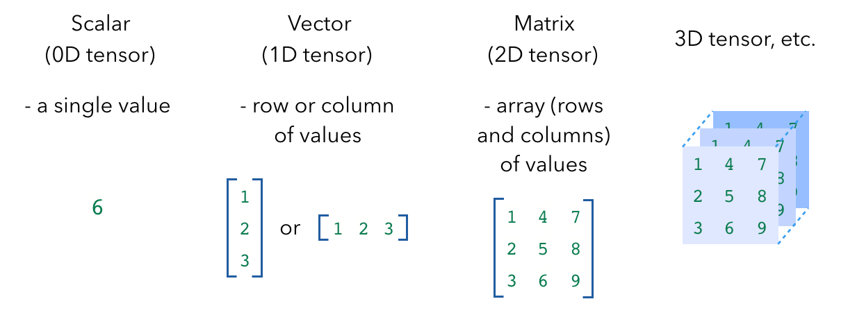
# Scalar
x = np.array(6)
print ("x: ", x)
print ("x ndim: ", x.ndim) # number of dimensions
print ("x shape:", x.shape) # dimensions
print ("x size: ", x.size) # size of elements
print ("x dtype: ", x.dtype) # data type
x: 6 x ndim: 0 x shape: () x size: 1 x dtype: int64
# Vector
x = np.array([1.3 , 2.2 , 1.7])
print ("x: ", x)
print ("x ndim: ", x.ndim)
print ("x shape:", x.shape)
print ("x size: ", x.size)
print ("x dtype: ", x.dtype) # notice the float datatype
x:  [1.3 2.2 1.7]
x ndim:  1
x shape: (3,)
x size:  3
x dtype:  float64
# Matrix
x = np.array([[1,2], [3,4]])
print ("x:\n", x)
print ("x ndim: ", x.ndim)
print ("x shape:", x.shape)
print ("x size: ", x.size)
print ("x dtype: ", x.dtype)
x:
 [[1 2]
 [3 4]]
x ndim:  2
x shape: (2, 2)
x size:  4
x dtype:  int64
# 3-D Tensor
x = np.array([[[1,2],[3,4]],[[5,6],[7,8]]])
print ("x:\n", x)
print ("x ndim: ", x.ndim)
print ("x shape:", x.shape)
print ("x size: ", x.size)
print ("x dtype: ", x.dtype)
x:
 [[[1 2]
  [3 4]]

 [[5 6]
  [7 8]]]
x ndim:  3
x shape: (2, 2, 2)
x size:  8
x dtype:  int64
NumPy 还带有几个函数,可以让我们快速创建张量。
# Functions
print ("np.zeros((2,2)):\n", np.zeros((2,2)))
print ("np.ones((2,2)):\n", np.ones((2,2)))
print ("np.eye((2)):\n", np.eye((2))) # identity matrix
print ("np.random.random((2,2)):\n", np.random.random((2,2)))
np.zeros((2,2)):
 [[0. 0.]
 [0. 0.]]
np.ones((2,2)):
 [[1. 1.]
 [1. 1.]]
np.eye((2)):
 [[1. 0.]
 [0. 1.]]
np.random.random((2,2)):
 [[0.19151945 0.62210877]
 [0.43772774 0.78535858]]
索引
我们可以使用索引从我们的张量中提取特定值。
请记住,索引行和列时,索引从
0. 和使用列表索引一样,我们也可以使用负索引(-1最后一项在哪里)。

# Indexing
x = np.array([1, 2, 3])
print ("x: ", x)
print ("x[0]: ", x[0])
x[0] = 0
print ("x: ", x)
x: [1 2 3] x[0]: 1 x: [0 2 3]
# Slicing
x = np.array([[1,2,3,4], [5,6,7,8], [9,10,11,12]])
print (x)
print ("x column 1: ", x[:, 1])
print ("x row 0: ", x[0, :])
print ("x rows 0,1 & cols 1,2: \n", x[0:2, 1:3])
[[ 1  2  3  4]
 [ 5  6  7  8]
 [ 9 10 11 12]]
x column 1:  [ 2  6 10]
x row 0:  [1 2 3 4]
x rows 0,1 & cols 1,2:
 [[2 3]
 [6 7]]
# Integer array indexing
print (x)
rows_to_get = np.array([0, 1, 2])
print ("rows_to_get: ", rows_to_get)
cols_to_get = np.array([0, 2, 1])
print ("cols_to_get: ", cols_to_get)
# Combine sequences above to get values to get
print ("indexed values: ", x[rows_to_get, cols_to_get]) # (0, 0), (1, 2), (2, 1)
[[ 1  2  3  4]
 [ 5  6  7  8]
 [ 9 10 11 12]]
rows_to_get:  [0 1 2]
cols_to_get:  [0 2 1]
indexed values:  [ 1  7 10]
# Boolean array indexing
x = np.array([[1, 2], [3, 4], [5, 6]])
print ("x:\n", x)
print ("x > 2:\n", x > 2)
print ("x[x > 2]:\n", x[x > 2])
x:
 [[1 2]
 [3 4]
 [5 6]]
x > 2:
 [[False False]
 [ True  True]
 [ True  True]]
x[x > 2]:
 [3 4 5 6]
算术
# Basic math
x = np.array([[1,2], [3,4]], dtype=np.float64)
y = np.array([[1,2], [3,4]], dtype=np.float64)
print ("x + y:\n", np.add(x, y)) # or x + y
print ("x - y:\n", np.subtract(x, y)) # or x - y
print ("x * y:\n", np.multiply(x, y)) # or x * y
x + y:
 [[2. 4.]
 [6. 8.]]
x - y:
 [[0. 0.]
 [0. 0.]]
x * y:
 [[ 1.  4.]
 [ 9. 16.]]
点积
我们将在机器学习中使用的最常见的 NumPy 运算之一是使用点积的矩阵乘法。假设我们想取两个形状为[2 X 3]和的矩阵的点积[3 X 2]。我们取第一个矩阵 (2) 的行和第二个矩阵 (2) 的列来确定点积,输出为[2 X 2]. 唯一的要求是内部尺寸匹配,在这种情况下,第一个矩阵有 3 列,第二个矩阵有 3 行。

# Dot product
a = np.array([[1,2,3], [4,5,6]], dtype=np.float64) # we can specify dtype
b = np.array([[7,8], [9,10], [11, 12]], dtype=np.float64)
c = a.dot(b)
print (f"{a.shape} · {b.shape} = {c.shape}")
print (c)
(2, 3) · (3, 2) = (2, 2)
[[ 58.  64.]
 [139. 154.]]
轴操作
我们还可以跨特定轴进行操作。

# Sum across a dimension
x = np.array([[1,2],[3,4]])
print (x)
print ("sum all: ", np.sum(x)) # adds all elements
print ("sum axis=0: ", np.sum(x, axis=0)) # sum across rows
print ("sum axis=1: ", np.sum(x, axis=1)) # sum across columns
[[1 2]
 [3 4]]
sum all:  10
sum axis=0:  [4 6]
sum axis=1:  [3 7]
# Min/max
x = np.array([[1,2,3], [4,5,6]])
print ("min: ", x.min())
print ("max: ", x.max())
print ("min axis=0: ", x.min(axis=0))
print ("min axis=1: ", x.min(axis=1))
min:  1
max:  6
min axis=0:  [1 2 3]
min axis=1:  [1 4]
播送
当我们尝试对形状看似不兼容的张量进行运算时会发生什么?它们的尺寸不兼容,但 NumPy 如何仍然给我们正确的结果?这就是广播的用武之地。标量通过向量进行广播,以便它们具有兼容的形状。
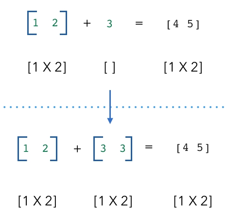
# Broadcasting
x = np.array([1,2]) # vector
y = np.array(3) # scalar
z = x + y
print ("z:\n", z)
z:
 [4 5]
陷阱
在下面的情况下,它的价值c和维度是什么?
a = np.array((3, 4, 5))
b = np.expand_dims(a, axis=1)
c = a + b
a.shape # (3,)
b.shape # (3, 1)
c.shape # (3, 3)
print (c)array([[ 6, 7, 8],
[ 7, 8, 9],
[ 8, 9, 10]])
我们如何解决这个问题?我们需要小心确保它a的形状与b我们不希望这种无意的广播行为相同。
a = a.reshape(-1, 1)
a.shape # (3, 1)
c = a + b
c.shape # (3, 1)
print (c)
array([[ 6],
       [ 8],
       [10]])
这种意外广播发生的频率比你想象的要多,因为这正是我们从列表创建数组时发生的情况。因此,我们需要确保在将其用于任何操作之前应用适当的重塑
a = np.array([3, 4, 5])
a.shape # (3,)
a = a.reshape(-1, 1)
a.shape # (3, 1)
转置
我们经常需要更改张量的维度以进行点积等操作。如果我们需要切换两个维度,我们可以转置张量。

# Transposing
x = np.array([[1,2,3], [4,5,6]])
print ("x:\n", x)
print ("x.shape: ", x.shape)
y = np.transpose(x, (1,0)) # flip dimensions at index 0 and 1
print ("y:\n", y)
print ("y.shape: ", y.shape)
x:
 [[1 2 3]
 [4 5 6]]
x.shape:  (2, 3)
y:
 [[1 4]
 [2 5]
 [3 6]]
y.shape:  (3, 2)
重塑(reshape)
有时,我们需要改变矩阵的维度。重塑允许我们将张量转换为不同的允许形状。下面,我们重塑的张量具有与原始张量相同数量的值。( 1X6= 2X3)。我们也可以-1在维度上使用,NumPy 将根据我们的输入张量推断维度。
# Reshaping
x = np.array([[1,2,3,4,5,6]])
print (x)
print ("x.shape: ", x.shape)
y = np.reshape(x, (2, 3))
print ("y: \n", y)
print ("y.shape: ", y.shape)
z = np.reshape(x, (2, -1))
print ("z: \n", z)
print ("z.shape: ", z.shape)
[[1 2 3 4 5 6]]
x.shape:  (1, 6)
y:
 [[1 2 3]
 [4 5 6]]
y.shape:  (2, 3)
z:
 [[1 2 3]
 [4 5 6]]
z.shape:  (2, 3)
reshape 的工作方式是查看新张量的每个维度,并将我们的原始张量分成那么多单元。所以这里新张量的索引 0 处的维度是 2,所以我们将原始张量分成 2 个单位,每个单位有 3 个值。

意外重塑
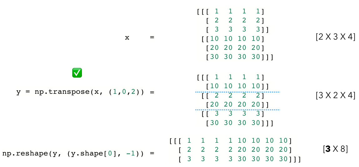
虽然重塑对于操纵张量非常方便,但我们也必须小心它的陷阱。让我们看看下面的例子。假设我们有x,其中有形状[2 X 3 X 4]。
x = np.array([[[1, 1, 1, 1], [2, 2, 2, 2], [3, 3, 3, 3]],
            [[10, 10, 10, 10], [20, 20, 20, 20], [30, 30, 30, 30]]])
print ("x:\n", x)
print ("x.shape: ", x.shape)
x: [[[ 1 1 1 1] [ 2 2 2 2] [ 3 3 3 3]]
[[10 10 10 10] .
[20 20 20 20]
[30 30 30 30]]]
x.shape: (2, 3, 4)
我们想要重塑 x 使其具有形状[3 X 8],但我们希望输出看起来像这样:
[[ 1  1  1  1 10 10 10 10]
[ 2  2  2  2 20 20 20 20]
[ 3  3  3  3 30 30 30 30]]
and not like:
[[ 1  1  1  1  2  2  2  2]
[ 3  3  3  3 10 10 10 10]
[20 20 20 20 30 30 30 30]]
我们想要重塑 x 使其具有形状[3 X 8],但我们希望输出看起来像这样:
当我们天真地进行重塑时,我们得到了正确的形状,但值并不是我们想要的。

# Unintended reshaping
z_incorrect = np.reshape(x, (x.shape[1], -1))
print ("z_incorrect:\n", z_incorrect)
print ("z_incorrect.shape: ", z_incorrect.shape)
z_incorrect:
[[ 1 1 1 1 2 2 2 2]
[ 3 3 3 3 10 10 10 10]
[20 20 20 20 30 30 30 30]]
z_incorrect.shape: (3, 8)
相反,如果我们转置张量然后进行整形,我们会得到我们想要的张量。Transpose 允许我们将我们想要组合的两个向量放在一起,然后我们使用 reshape 将它们连接在一起。作为一般规则,我们应该始终将我们的维度放在一起,然后再重新塑造以组合它们。
# Intended reshaping
y = np.transpose(x, (1,0,2))
print ("y:\n", y)
print ("y.shape: ", y.shape)
z_correct = np.reshape(y, (y.shape[0], -1))
print ("z_correct:\n", z_correct)
print ("z_correct.shape: ", z_correct.shape)
和:
[[[ 1 1 1 1]
[10 10 10 10]]
[[ 2 2 2 2] [20 20 20 20]]
[[ 3 3 3 3] [30 30 30 30]]]
y.shape: (3, 2, 4)
z_correct: [[ 1 1 1 1 10 10 10 10]
[ 2 2 2 2 20 20 20 20]
[ 3 3 3 3 30 30 30 30]]
z_correct.shape: (3, 8)
当我们在许多机器学习任务中处理具有随机值的权重张量时,这变得很困难。所以一个好主意是当你不确定重塑时总是创建一个像这样的虚拟示例。盲目地使用张量形状可能会导致很多下游问题。
Joining
x = np.random.random((2, 3))
print (x)
print (x.shape)
[[0.79564718 0.73023418 0.92340453] [0.24929281 0.0513762 0.66149188]] (2, 3)
# Concatenation
y = np.concatenate([x, x], axis=0) # concat on a specified axis
print (y)
print (y.shape)
[[0.79564718 0.73023418 0.92340453] [0.24929281 0.0513762 0.66149188] [0.79564718 0.73023418 0.92340453] [0.24929281 0.0513762 0.66149188]] (4, 3)
# Stacking
z = np.stack([x, x], axis=0) # stack on new axis
print (z)
print (z.shape)
[[[0.79564718 0.73023418 0.92340453] [0.24929281 0.0513762 0.66149188]] [[0.79564718 0.73023418 0.92340453] [0.24929281 0.0513762 0.66149188]]] (2, 2, 3)
扩大/缩小
我们还可以轻松地为我们的张量添加和删除维度,我们希望这样做以使张量与某些操作兼容。
# Adding dimensions
x = np.array([[1,2,3],[4,5,6]])
print ("x:\n", x)
print ("x.shape: ", x.shape)
y = np.expand_dims(x, 1) # expand dim 1
print ("y: \n", y)
print ("y.shape: ", y.shape)   # notice extra set of brackets are added
x:
 [[1 2 3]
  [4 5 6]]
x.shape:  (2, 3)
y:
 [[[1 2 3]]
  [[4 5 6]]]
y.shape:  (2, 1, 3)
# Removing dimensions
x = np.array([[[1,2,3]],[[4,5,6]]])
print ("x:\n", x)
print ("x.shape: ", x.shape)
y = np.squeeze(x, 1) # squeeze dim 1
print ("y: \n", y)
print ("y.shape: ", y.shape)  # notice extra set of brackets are gone
x:
 [[[1 2 3]]
  [[4 5 6]]]
x.shape:  (2, 1, 3)
y:
 [[1 2 3]
  [4 5 6]]
y.shape:  (2, 3)
查看Dask以扩展 NumPy 工作流,只需对现有代码进行最少的更改
相关文章
- 李宏毅《机器学习》丨4. Deep Learning(深度学习)
- 机器视觉应用方向及学习思路总结
- 机器学习入门 3-10 Numpy中的比较和Fancy Indexing
- 甲骨文机器更换IP地址
- Jeff Dean:机器学习在硬件设计中的潜力
- 中国 AI 市场格局(计算机视觉:商汤、旷视、海康)(语音语义:讯飞、阿里、百度)(机器学习平台:第四范式、华为、九章云极)
- 图灵奖得主Judea Pearl谈机器学习:不能只靠数据
- NLP 发展如何?机器之心 SOTA 模型库、知识库告诉你答案
- OpenAI再获100亿美元?DoNotPay力砸100万仅为AI律师辩护复述;新冠四种亚型被机器学习算法进行归纳
- 预测友谊和其他有趣的图机器学习任务
- ssh 与远程机器保持心跳(linux)详解程序员
- 机器学习之特征归一化(normalization)详解大数据
- 读写性能Redis集群中单数台机器的读写性能提升(redis集群单数台)