基于独立分量分析进行模态分解（Matlab代码实现）

 👨‍🎓个人主页：研学社的博客 

💥💥💞💞欢迎来到本博客❤️❤️💥💥

🏆博主优势：🌞🌞🌞博客内容尽量做到思维缜密，逻辑清晰，为了方便读者。

⛳️座右铭：行百里者，半于九十。

📋📋📋本文目录如下：🎁🎁🎁

目录

💥1 概述

📚2 运行结果

🌈3 Matlab代码实现

🎉4 参考文献

---

💥1 概述

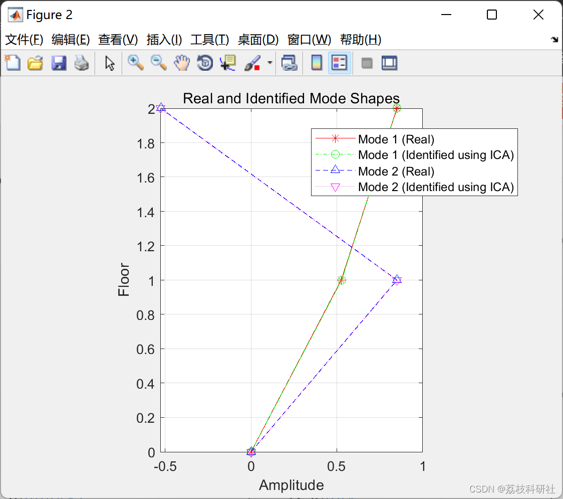
本文使用脉冲激励下的 2DOF 系统的独立分量分析 （ICA） 识别振型。

📚2 运行结果

🌈3 Matlab代码实现

部分代码：

zeta=Cn./(sqrt(2.*Mn.*Kn));  % damping ratio
wd=wn.*sqrt(1-zeta.^2);

fn=Vectors'*f; % generalized input force matrix

t=[0:dt:dt*steps-dt];

for i=1:1:n
    
    h(i,:)=(1/(Mn(i)*wd(i))).*exp(-zeta(i)*wn(i)*t).*sin(wd(i)*t); %transfer function of displacement
    hd(i,:)=(1/(Mn(i)*wd(i))).*(-zeta(i).*wn(i).*exp(-zeta(i)*wn(i)*t).*sin(wd(i)*t)+wd(i).*exp(-zeta(i)*wn(i)*t).*cos(wd(i)*t)); %transfer function of velocity
    hdd(i,:)=(1/(Mn(i)*wd(i))).*((zeta(i).*wn(i))^2.*exp(-zeta(i)*wn(i)*t).*sin(wd(i)*t)-zeta(i).*wn(i).*wd(i).*exp(-zeta(i)*wn(i)*t).*cos(wd(i)*t)-wd(i).*((zeta(i).*wn(i)).*exp(-zeta(i)*wn(i)*t).*cos(wd(i)*t))-wd(i)^2.*exp(-zeta(i)*wn(i)*t).*sin(wd(i)*t)); %transfer function of acceleration
    
    qq=conv(fn(i,:),h(i,:))*dt;
    qqd=conv(fn(i,:),hd(i,:))*dt;
    qqdd=conv(fn(i,:),hdd(i,:))*dt;
    
    q(i,:)=qq(1:steps); % modal displacement
    qd(i,:)=qqd(1:steps); % modal velocity
    qdd(i,:)=qqdd(1:steps); % modal acceleration
       
end

x=Vectors*q; %displacement
v=Vectors*qd; %vecloity
a=Vectors*qdd; %vecloity

%Add noise to excitation and response
%--------------------------------------------------------------------------
f2=f+0.0*randn(2,10000);
a2=a+0.0*randn(2,10000);
v2=v+0.0*randn(2,10000);
x2=x+0.0*randn(2,10000);

%Plot displacement of first floor without and with noise
%--------------------------------------------------------------------------
figure;
subplot(3,2,1)
plot(t,f(1,:)); xlabel('Time (sec)');  ylabel('Force1'); title('First Floor');
subplot(3,2,2)
plot(t,f(2,:)); xlabel('Time (sec)');  ylabel('Force2'); title('Second Floor');
subplot(3,2,3)
plot(t,x(1,:)); xlabel('Time (sec)');  ylabel('DSP1');
subplot(3,2,4)
plot(t,x(2,:)); xlabel('Time (sec)');  ylabel('DSP2');
subplot(3,2,5)
plot(t,x2(1,:)); xlabel('Time (sec)');  ylabel('DSP1+Noise');
subplot(3,2,6)
plot(t,x2(2,:)); xlabel('Time (sec)');  ylabel('DSP2+Noise');

%Identify modal parameters using displacement with added uncertainty
%--------------------------------------------------------------------------
Mdl = rica(x2',n);            %ICA 
V=Mdl.TransformWeights;
V(:,1)=V(:,1)/sign(V(1,1));
V(:,2)=V(:,2)/sign(V(1,2));

%Plot real and identified first modes to compare between them
%--------------------------------------------------------------------------
figure;
plot([0 ; -Vectors(:,1)],[0 1 2],'r*-');
hold on
plot([0  ;V(:,1)],[0 1 2],'go-.');
hold on
plot([0 ; -Vectors(:,2)],[0 1 2],'b^--');
hold on
plot([0  ;V(:,2)],[0 1 2],'mv:');
hold off
title('Real and Identified Mode Shapes');
legend('Mode 1 (Real)','Mode 1 (Identified using ICA)','Mode 2 (Real)','Mode 2 (Identified using ICA)');
xlabel('Amplitude');

🎉4 参考文献

部分理论来源于网络，如有侵权请联系删除。

[1] Al Rumaithi, Ayad, "Characterization of Dynamic Structures Using Parametric and Non-parametric System Identification Methods" (2014). Electronic Theses and Dissertations. 1325.

[2] Al-Rumaithi, Ayad, Hae-Bum Yun, and Sami F. Masri. "A Comparative Study of Mode Decomposition to Relate Next-ERA, PCA, and ICA Modes." Model Validation and Uncertainty Quantification, Volume 3. Springer, Cham, 2015. 113-133.