
ML之shap:基于adult人口普查收入二分类预测数据集(预测年收入是否超过50k)利用shap决策图结合LightGBM模型实现异常值检测案例之详细攻略
2023-09-14 09:04:44 时间
ML之shap:基于adult人口普查收入二分类预测数据集(预测年收入是否超过50k)利用shap决策图结合LightGBM模型实现异常值检测案例之详细攻略
目录
基于adult人口普查收入二分类预测数据集(预测年收入是否超过50k)利用shap决策图结合LightGBM模型实现异常值检测案例之详细攻略
相关文章
Dataset:adult人口普查收入二分类预测数据集(预测年收入是否超过50k)的简介、下载、使用方法之详细攻略
ML之shap:基于adult人口普查收入二分类预测数据集(预测年收入是否超过50k)利用shap决策图结合LightGBM模型实现异常值检测案例之详细攻略
ML之shap:基于adult人口普查收入二分类预测数据集(预测年收入是否超过50k)利用shap决策图结合LightGBM模型实现异常值检测案例之详细攻略实现
基于adult人口普查收入二分类预测数据集(预测年收入是否超过50k)利用shap决策图结合LightGBM模型实现异常值检测案例之详细攻略
# 1、定义数据集
| age | workclass | fnlwgt | education | education_num | marital_status | occupation | relationship | race | sex | capital_gain | capital_loss | hours_per_week | native_country | salary |
| 39 | State-gov | 77516 | Bachelors | 13 | Never-married | Adm-clerical | Not-in-family | White | Male | 2174 | 0 | 40 | United-States | <=50K |
| 50 | Self-emp-not-inc | 83311 | Bachelors | 13 | Married-civ-spouse | Exec-managerial | Husband | White | Male | 0 | 0 | 13 | United-States | <=50K |
| 38 | Private | 215646 | HS-grad | 9 | Divorced | Handlers-cleaners | Not-in-family | White | Male | 0 | 0 | 40 | United-States | <=50K |
| 53 | Private | 234721 | 11th | 7 | Married-civ-spouse | Handlers-cleaners | Husband | Black | Male | 0 | 0 | 40 | United-States | <=50K |
| 28 | Private | 338409 | Bachelors | 13 | Married-civ-spouse | Prof-specialty | Wife | Black | Female | 0 | 0 | 40 | Cuba | <=50K |
| 37 | Private | 284582 | Masters | 14 | Married-civ-spouse | Exec-managerial | Wife | White | Female | 0 | 0 | 40 | United-States | <=50K |
| 49 | Private | 160187 | 9th | 5 | Married-spouse-absent | Other-service | Not-in-family | Black | Female | 0 | 0 | 16 | Jamaica | <=50K |
| 52 | Self-emp-not-inc | 209642 | HS-grad | 9 | Married-civ-spouse | Exec-managerial | Husband | White | Male | 0 | 0 | 45 | United-States | >50K |
| 31 | Private | 45781 | Masters | 14 | Never-married | Prof-specialty | Not-in-family | White | Female | 14084 | 0 | 50 | United-States | >50K |
| 42 | Private | 159449 | Bachelors | 13 | Married-civ-spouse | Exec-managerial | Husband | White | Male | 5178 | 0 | 40 | United-States | >50K |
# 2、数据集预处理
# 2.1、入模特征初步筛选
df.columns
14
# 2.2、目标特征二值化
# 2.3、类别型特征编码数字化
| age | workclass | education_num | marital_status | occupation | relationship | race | sex | capital_gain | capital_loss | hours_per_week | native_country | salary | |
| 0 | 39 | 7 | 13 | 4 | 1 | 1 | 4 | 1 | 2174 | 0 | 40 | 39 | 0 |
| 1 | 50 | 6 | 13 | 2 | 4 | 0 | 4 | 1 | 0 | 0 | 13 | 39 | 0 |
| 2 | 38 | 4 | 9 | 0 | 6 | 1 | 4 | 1 | 0 | 0 | 40 | 39 | 0 |
| 3 | 53 | 4 | 7 | 2 | 6 | 0 | 2 | 1 | 0 | 0 | 40 | 39 | 0 |
| 4 | 28 | 4 | 13 | 2 | 10 | 5 | 2 | 0 | 0 | 0 | 40 | 5 | 0 |
| 5 | 37 | 4 | 14 | 2 | 4 | 5 | 4 | 0 | 0 | 0 | 40 | 39 | 0 |
| 6 | 49 | 4 | 5 | 3 | 8 | 1 | 2 | 0 | 0 | 0 | 16 | 23 | 0 |
| 7 | 52 | 6 | 9 | 2 | 4 | 0 | 4 | 1 | 0 | 0 | 45 | 39 | 1 |
| 8 | 31 | 4 | 14 | 4 | 10 | 1 | 4 | 0 | 14084 | 0 | 50 | 39 | 1 |
| 9 | 42 | 4 | 13 | 2 | 4 | 0 | 4 | 1 | 5178 | 0 | 40 | 39 | 1 |
# 2.4、分离特征与标签
| age | workclass | education_num | marital_status | occupation | relationship | race | sex | capital_gain | capital_loss | hours_per_week | native_country |
| 39 | 7 | 13 | 4 | 1 | 1 | 4 | 1 | 2174 | 0 | 40 | 39 |
| 50 | 6 | 13 | 2 | 4 | 0 | 4 | 1 | 0 | 0 | 13 | 39 |
| 38 | 4 | 9 | 0 | 6 | 1 | 4 | 1 | 0 | 0 | 40 | 39 |
| 53 | 4 | 7 | 2 | 6 | 0 | 2 | 1 | 0 | 0 | 40 | 39 |
| 28 | 4 | 13 | 2 | 10 | 5 | 2 | 0 | 0 | 0 | 40 | 5 |
| 37 | 4 | 14 | 2 | 4 | 5 | 4 | 0 | 0 | 0 | 40 | 39 |
| 49 | 4 | 5 | 3 | 8 | 1 | 2 | 0 | 0 | 0 | 16 | 23 |
| 52 | 6 | 9 | 2 | 4 | 0 | 4 | 1 | 0 | 0 | 45 | 39 |
| 31 | 4 | 14 | 4 | 10 | 1 | 4 | 0 | 14084 | 0 | 50 | 39 |
| 42 | 4 | 13 | 2 | 4 | 0 | 4 | 1 | 5178 | 0 | 40 | 39 |
| salary |
| 0 |
| 0 |
| 0 |
| 0 |
| 0 |
| 0 |
| 0 |
| 1 |
| 1 |
| 1 |
#3、模型训练与推理
# 3.1、数据集切分
X_test
| age | workclass | education_num | marital_status | occupation | relationship | race | sex | capital_gain | capital_loss | hours_per_week | native_country | |
| 1342 | 47 | 3 | 10 | 0 | 1 | 1 | 4 | 1 | 0 | 0 | 40 | 35 |
| 1338 | 71 | 3 | 13 | 0 | 13 | 3 | 4 | 0 | 2329 | 0 | 16 | 35 |
| 189 | 58 | 6 | 16 | 2 | 10 | 0 | 4 | 1 | 0 | 0 | 1 | 35 |
| 1332 | 23 | 3 | 9 | 4 | 7 | 1 | 2 | 1 | 0 | 0 | 35 | 35 |
| 1816 | 46 | 2 | 9 | 2 | 3 | 0 | 4 | 1 | 0 | 1902 | 40 | 35 |
| 1685 | 37 | 3 | 9 | 2 | 4 | 0 | 4 | 1 | 0 | 1902 | 45 | 35 |
| 657 | 34 | 3 | 9 | 2 | 3 | 0 | 4 | 1 | 0 | 0 | 45 | 35 |
| 1846 | 21 | 0 | 10 | 4 | 0 | 3 | 4 | 0 | 0 | 0 | 40 | 35 |
| 554 | 33 | 1 | 11 | 0 | 3 | 4 | 2 | 0 | 0 | 0 | 40 | 35 |
| 1963 | 49 | 3 | 13 | 2 | 12 | 0 | 4 | 1 | 0 | 0 | 50 | 35 |
# 3.2、模型建立并训练
params = {
    "max_bin": 512, "learning_rate": 0.05,
    "boosting_type": "gbdt", "objective": "binary",
    "metric": "binary_logloss", "verbose": -1,
     "min_data": 100, "random_state": 1,
    "boost_from_average": True, "num_leaves": 10 }

LGBMC = lgb.train(params, lgbD_train, 10000,
                  valid_sets=[lgbD_test],
                  early_stopping_rounds=50,
                  verbose_eval=1000)
# 3.3、模型预测
| age | workclass | education_num | marital_status | occupation | relationship | race | sex | capital_gain | capital_loss | hours_per_week | native_country | y_test_predi | y_test | |
| 1342 | 47 | 3 | 10 | 0 | 1 | 1 | 4 | 1 | 0 | 0 | 40 | 35 | 0.045225575 | 0 |
| 1338 | 71 | 3 | 13 | 0 | 13 | 3 | 4 | 0 | 2329 | 0 | 16 | 35 | 0.074799172 | 0 |
| 189 | 58 | 6 | 16 | 2 | 10 | 0 | 4 | 1 | 0 | 0 | 1 | 35 | 0.30014332 | 1 |
| 1332 | 23 | 3 | 9 | 4 | 7 | 1 | 2 | 1 | 0 | 0 | 35 | 35 | 0.003966427 | 0 |
| 1816 | 46 | 2 | 9 | 2 | 3 | 0 | 4 | 1 | 0 | 1902 | 40 | 35 | 0.363861294 | 0 |
| 1685 | 37 | 3 | 9 | 2 | 4 | 0 | 4 | 1 | 0 | 1902 | 45 | 35 | 0.738628671 | 1 |
| 657 | 34 | 3 | 9 | 2 | 3 | 0 | 4 | 1 | 0 | 0 | 45 | 35 | 0.376412174 | 0 |
| 1846 | 21 | 0 | 10 | 4 | 0 | 3 | 4 | 0 | 0 | 0 | 40 | 35 | 0.002309884 | 0 |
| 554 | 33 | 1 | 11 | 0 | 3 | 4 | 2 | 0 | 0 | 0 | 40 | 35 | 0.060345836 | 1 |
| 1963 | 49 | 3 | 13 | 2 | 12 | 0 | 4 | 1 | 0 | 0 | 50 | 35 | 0.703506366 | 1 |
# 4、利用shap决策图进行异常值检测
# 4.1、原始数据和预处理后的数据各采样一小部分样本
# 4.2、创建Explainer并计算SHAP值
shap2exp.values.shape (100, 12, 2)
 [[[-5.97178729e-01  5.97178729e-01]
  [-5.18879297e-03  5.18879297e-03]
  [ 1.70566444e-01 -1.70566444e-01]
  ...
  [ 0.00000000e+00  0.00000000e+00]
  [ 6.58794799e-02 -6.58794799e-02]
  [ 0.00000000e+00  0.00000000e+00]]

 [[-4.45574118e-01  4.45574118e-01]
  [-1.00665452e-03  1.00665452e-03]
  [-8.12237233e-01  8.12237233e-01]
  ...
  [ 0.00000000e+00  0.00000000e+00]
  [ 8.56381961e-01 -8.56381961e-01]
  [ 0.00000000e+00  0.00000000e+00]]

 [[-3.87412165e-01  3.87412165e-01]
  [ 1.52848351e-01 -1.52848351e-01]
  [-1.02755954e+00  1.02755954e+00]
  ...
  [ 0.00000000e+00  0.00000000e+00]
  [ 1.10240434e+00 -1.10240434e+00]
  [ 0.00000000e+00  0.00000000e+00]]

 ...

 [[-5.28928223e-01  5.28928223e-01]
  [ 7.14116015e-03 -7.14116015e-03]
  [-8.82241728e-01  8.82241728e-01]
  ...
  [ 0.00000000e+00  0.00000000e+00]
  [ 7.47521189e-02 -7.47521189e-02]
  [ 0.00000000e+00  0.00000000e+00]]

 [[ 2.20002984e+00 -2.20002984e+00]
  [ 7.75916086e-03 -7.75916086e-03]
  [ 3.95152810e-01 -3.95152810e-01]
  ...
  [ 0.00000000e+00  0.00000000e+00]
  [ 1.52566789e-01 -1.52566789e-01]
  [ 0.00000000e+00  0.00000000e+00]]

 [[-8.28965461e-01  8.28965461e-01]
  [-4.43687947e-02  4.43687947e-02]
  [ 3.37305776e-01 -3.37305776e-01]
  ...
  [ 0.00000000e+00  0.00000000e+00]
  [ 8.26477289e-03 -8.26477289e-03]
  [ 0.00000000e+00  0.00000000e+00]]]
shap2array.shape (100, 12)
LightGBM binary classifier with TreeExplainer shap values output has changed to a list of ndarray
 [[ 5.97178729e-01  5.18879297e-03 -1.70566444e-01 ...  0.00000000e+00
  -6.58794799e-02  0.00000000e+00]
 [ 4.45574118e-01  1.00665452e-03  8.12237233e-01 ...  0.00000000e+00
  -8.56381961e-01  0.00000000e+00]
 [ 3.87412165e-01 -1.52848351e-01  1.02755954e+00 ...  0.00000000e+00
  -1.10240434e+00  0.00000000e+00]
 ...
 [ 5.28928223e-01 -7.14116015e-03  8.82241728e-01 ...  0.00000000e+00
  -7.47521189e-02  0.00000000e+00]
 [-2.20002984e+00 -7.75916086e-03 -3.95152810e-01 ...  0.00000000e+00
  -1.52566789e-01  0.00000000e+00]
 [ 8.28965461e-01  4.43687947e-02 -3.37305776e-01 ...  0.00000000e+00
  -8.26477289e-03  0.00000000e+00]]
mode_exp_value: -1.9982244224656025
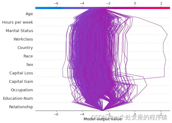
# 4.3、shap决策图可视化
# 将决策图叠加在一起有助于根据shap定位异常值,即偏离密集群处的样本
相关文章
- robotframework案例
- 无线ldap认证服务器,结合LDAP服务器进行portal认证配置案例
- 故障分析 | 从一则 MGR 异常切换案例,看系统时间对 MGR 的影响
- 系统架构师、分析师2023年案例分析考前冲刺
- 【Java 代码审计入门-05】RCE 漏洞原理与实际案例介绍
- Linux内核的内存管理与漏洞利用案例分析
- 蓝牙安全与攻击案例分析
- NLP自然语言处理—主题模型LDA案例:挖掘人民网留言板文本数据|附代码数据
- Golang 上下文 Context 通过案例讲源码(1): 值传递
- SAMBA实战案例:实现不同samba用户访问相同的samba共享,实现不同的配置
- Oracle RAC全解析:深度剖析Oracle RAC技术,实战案例详解,助您轻松掌握!(oraclerac书籍)
- Redis读写分离从案例中学习运用(redis读写分离案例)
- MongoDB查询字段没有创建索引导致的连接超时异常解案例分享