覆盖和覆盖D2D通信网络的传输容量分析（Matlab代码实现）

           目录

💥1 概述

📚2 运行结果

🎉3 参考文献

👨‍💻4 Matlab代码

💥1 概述

移动数据流量的日益增长与有限的频谱资源之间的矛盾催生了用以提升频谱空间利用率的设备到设备（Device-to-Device,D2D）通信技术。在D2D通信技术中,邻近设备之间直接进行数据通信,而无需基站（Base Station,BS）参与中转。与传统的蜂窝通信方式相比,D2D通信技术显著地缩短了通信距离,有效地提升了数据传输速率、频谱效率及频谱空间利用率,极大地降低了传输延时、传输功耗及BS的流量负载。因此,D2D通信技术被认为是5G后时代（Beyond Fifth-Generation,B5G）移动通信系统的关键使能技术之一。现有研究发现,D2D通信技术尤其适用于高速率、低延时要求的视频通信场景。但实现D2D网络中的高效视频传输,仍然需要解决三个关键性问题:1)D2D网络中用户需求多元、终端设备多样、无线信道多变,对于视频编码的可伸缩性、灵活性和简单性提出了很高的要求。2)海量视频数据的传输对网络资源的超高需求与网络资源多样、分散、利用率低的现状存在矛盾,需要对网络资源进行全面的协调和综合的调度。3)用户设备的随机接入和断开、用户的移动性和自私性导致D2D协作通常难以实施,需要一个兼具公平性和激励性的协作机制来促进协作的开展和视频内容的分享。

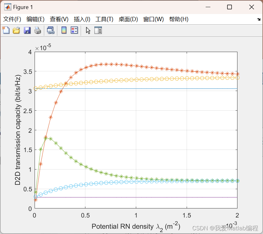
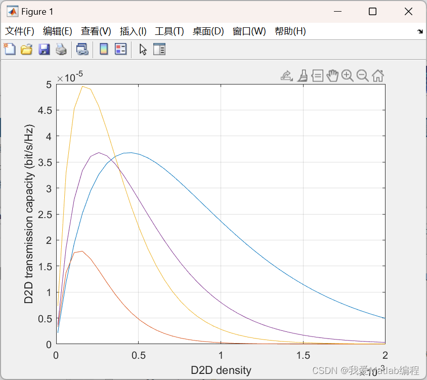
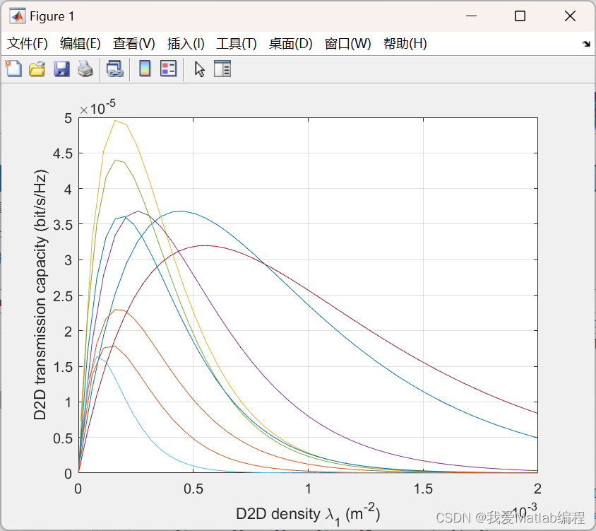
📚2 运行结果

🎉3 参考文献

[1]张旭光. 面向D2D网络的视频通信技术研究[D].南京邮电大学,2021.DOI:10.27251/d.cnki.gnjdc.2021.001609.

👨‍💻4 Matlab代码

主函数部分代码：

%% Program init
clear;
clc;
close all;
format long g;

%% Try genetic algo for 2 vars

% lambda2 vs P2 vs error function (constraint function) graph, as a surface
% plot.
syms x y;
ezsurf(constraint_func([x y]), [0.0001, 0.0009, 0.006309, 0.1]);
title('TC - Target as a function of \lambda_{2} and P2')

ObjectiveFunction = @fitness_func;
nvars = 2;    % Number of variables
LB = [0.0001 0.006309];   % Lower bound
UB = [0.0009 0.1];  % Upper bound
ConstraintFunction = @constraint_func;
options=gaoptimset('PopulationSize',80,'Generations',400,'StallGenLimit',200,'SelectionFcn', @selectionroulette,'CrossoverFcn',@crossovertwopoint,'Display', 'off');
[x,fval] = ga(ObjectiveFunction,nvars,[],[],[],[],LB,UB, ...
    ConstraintFunction, options);

fprintf("TC = %g bps/Hz \n", tc(0.0001, 0.0003,x(1),24, 15, 10*log10(x(2)) + 30, 0,2,2, 4, 35));
fprintf("RN Tx power = %g dBm \n", 10*log10(x(2)) + 30);
fprintf("RN density (# of relay nodes/ Km^2) = %g \n", x(1)*1e6);
fprintf("Output RNPD = %g W/Km2 \n", x(2) * x(1) * 1e6);

% Fitness function is what is to be minimized
function y = fitness_func(V)
    % Try and minimize the Tx power/ unit area for the RN.

    
    l2 = V(1);
    P2 = V(2);

      y = (l2*P2*1e6)^2;
end

function [c, ceq] = constraint_func(V)
    
    l2 = V(1);
    p2 = V(2);
    
    p2 = 10*log10(p2) + 30; % converting to dBm for the TC code
    % Here "target" is the TC that we want for that area, therefore, a
    % constraint
    target = 6; % bps/Hz * 1e6, scaled as this resulted in better optimisation outputs
    c = [(tc(0.0001, 0.0003,l2,24, 15, p2, 0,2,2, 4, 35)*1e6 - target)^2];
    ceq = [];
end