过滤 ：是信号和图像处理中基本的任务。其目的是根据应用环境的不同，选择性的提取图像中某些认为是重要的信息。过滤可以移除图像中的噪音、提取感兴趣的可视特征、允许图像重采样等等。

频域分析 ：将图像分成从低频到高频的不同部分。低频对应图像强度变化小的区域，而高频是图像强度变化非常大的区域。

在频率分析领域的框架中，滤波器是一个用来增强图像中某个波段或频率并阻塞（或降低）其他频率波段的操作。低通滤波器是消除图像中高频部分，但保留低频部分。高通滤波器消除低频部分。

滤波(高通、低通、带通、带阻) 、模糊、去噪、平滑等。
 

图像在频域里面，频率低的地方说明它是比较平滑的，因为平滑的地方灰度值变化比较小，而频率高的地方通常是边缘或者噪声，因为这些地方往往是灰度值突变的。

• 所谓高通滤波就是保留频率比较高的部分，即突出边缘；
• 低通滤波就是保留频率比较低的地方，即平滑图像，弱化边缘，消除噪声。

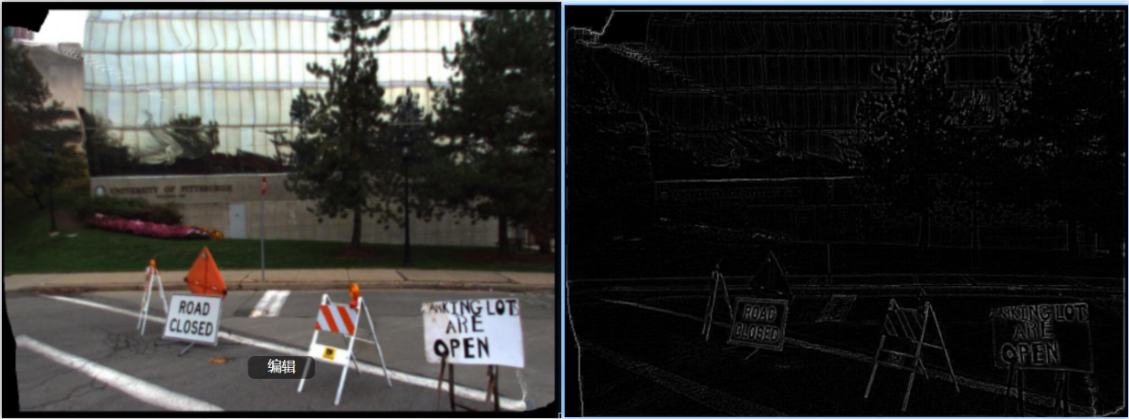
实现sobel算子的卷积操作（提取边缘轮廓）

在pytorch中实现将sobel算子和卷积层结合来提取图像中物体的边缘轮廓图，如下代码是卷积执行soble边缘检测算子的实现：

import torch
import numpy as np
from torch import nn
from PIL import Image
from torch.autograd import Variable
import torch.nn.functional as F

# https://blog.csdn.net/weicao1990/article/details/100521530 
 
def nn_conv2d(im):
    # 用nn.Conv2d定义卷积操作
    conv_op = nn.Conv2d(1, 1, 3, bias=False)
    # 定义sobel算子参数
    sobel_kernel = np.array([[-1, -1, -1], [-1, 8, -1], [-1, -1, -1]], dtype='float32')
    # 将sobel算子转换为适配卷积操作的卷积核
    sobel_kernel = sobel_kernel.reshape((1, 1, 3, 3))
    # 给卷积操作的卷积核赋值
    conv_op.weight.data = torch.from_numpy(sobel_kernel)
    # 对图像进行卷积操作
    edge_detect = conv_op(Variable(im))
    # 将输出转换为图片格式
    edge_detect = edge_detect.squeeze().detach().numpy()
    return edge_detect
 
def functional_conv2d(im):
    sobel_kernel = np.array([[-1, -1, -1], [-1, 8, -1], [-1, -1, -1]], dtype='float32')  #
    sobel_kernel = sobel_kernel.reshape((1, 1, 3, 3))
    weight = Variable(torch.from_numpy(sobel_kernel))
    edge_detect = F.conv2d(Variable(im), weight)
    edge_detect = edge_detect.squeeze().detach().numpy()
    return edge_detect
 
def main():
    # 读入一张图片，并转换为灰度图
    im = Image.open('./cat.jpg').convert('L')
    # 将图片数据转换为矩阵
    im = np.array(im, dtype='float32')
    # 将图片矩阵转换为pytorch tensor,并适配卷积输入的要求
    im = torch.from_numpy(im.reshape((1, 1, im.shape[0], im.shape[1])))
    # 边缘检测操作
    # edge_detect = nn_conv2d(im)
    edge_detect = functional_conv2d(im)
    # 将array数据转换为image
    im = Image.fromarray(edge_detect)
    # image数据转换为灰度模式
    im = im.convert('L')
    # 保存图片
    im.save('edge.jpg', quality=95)
 
if __name__ == "__main__":
    main()

效果展示： 

使用不同的卷积滤波核（sobal、average、Gaussian、Laplace）

四种算子：

• sobel_Gy = [[-1,0,1],[-2,0,2],[-1,0,1]]
• Average = [[1/9,1/9,1/9],[1/9,1/9,1/9],[1/9,1/9,1/9]]
• Gaussian = [[1/16,2/16,1/16],[2/16,4/16,2/16],[1/16,2/16,1/16]]
• Laplace = [[-1,-1,-1],[-1,9,-1],[-1,-1,-1]] 

'''
滤波与卷积
'''
# https://blog.csdn.net/m0_43609475/article/details/112447397

import cv2
import numpy as np
import matplotlib.pyplot as plt

def Padding(image,kernels_size,stride = [1,1],padding = "same"):
    '''
    对图像进行padding
    :param image: 要padding的图像矩阵
    :param kernels_size: list 卷积核大小[h,w]
    :param stride: 卷积步长 [左右步长，上下步长]
    :param padding: padding方式
    :return: padding后的图像
    '''
    if padding == "same":
        h,w = image.shape
        p_h =max((stride[0]*(h-1)-h+kernels_size[0]),0)  # 高度方向要补的0
        p_w =max((stride[1]*(w-1)-w+kernels_size[1]),0)  # 宽度方向要补的0
        p_h_top = p_h//2                                 # 上边要补的0
        p_h_bottom = p_h-p_h_top                         # 下边要补的0
        p_w_left = p_w//2                                # 左边要补的0
        p_w_right = p_w-p_w_left                         # 右边要补的0
        # print(p_h_top,p_h_bottom,p_w_left,p_w_right)     # 输出padding方式
        padding_image = np.zeros((h+p_h, w+p_w), dtype=np.uint8)
        for i in range(h):
            for j in range(w):
                    padding_image[i+p_h_top][j+p_w_left] = image[i][j] # 将原来的图像放入新图中做padding
        return padding_image
    else:
        return image


def filtering_and_convolution(image,kernels,stride,padding = "same"):
    '''
    :param image: 要卷积的图像
    :param kernels: 卷积核 列表
    :param stride: 卷积步长 [左右步长，上下步长]
    :param padding: padding方式 “same”or“valid”
    :return:
    '''
    image_h,image_w = image.shape
    kernels_h,kernels_w = np.array(kernels).shape
    # 获取卷积核的中心点
    kernels_h_core = int(kernels_h/2+0.5)-1
    kernels_w_core = int(kernels_w/2+0.5)-1
    if padding == "valid":
        # 计算卷积后的图像大小
        h = int((image_h-kernels_h)/stride[0]+1)
        w = int((image_w-kernels_w)/stride[1]+1)
        # 生成卷积后的图像
        conv_image = np.zeros((h,w),dtype=np.uint8)
        # 计算遍历起始点
        h1_start = kernels_h//2
        w1_start = kernels_w//2
        ii=-1
        for i in range(h1_start,image_h - h1_start,stride[0]):
            ii += 1
            jj = 0
            for j in range(w1_start,image_w - w1_start,stride[1]):
                sum = 0
                for x in range(kernels_h):
                    for y in range(kernels_w):
                        # print(i,j,int((i/image_h)*h),int((j/image_w)*w),  i-kernels_h_core + x,  j-kernels_w_core+y,x,y)
                        sum += int(image[i-kernels_h_core+x][j-kernels_w_core+y]*kernels[x][y])
                conv_image[ii][jj] = sum
                jj += 1
        return conv_image

    if padding == "same":
        # 对原图进行padding
        kernels_size = [kernels_h, kernels_w]
        pad_image = Padding(image,kernels_size,stride,padding="same")
        # 计算卷积后的图像大小
        h = image_h
        w = image_w
        # 生成卷积后的图像
        conv_image = np.zeros((h,w),dtype=np.uint8)
        # # 计算遍历起始点
        h1_start = kernels_h//2
        w1_start = kernels_w//2
        ii=-1
        for i in range(h1_start,image_h - h1_start,stride[0]):
            ii +=1
            jj = 0
            for j in range(w1_start,image_w - w1_start,stride[1]):
                sum = 0
                for x in range(kernels_h):
                    for y in range(kernels_w):
                        sum += int(image[i-kernels_h_core+x][j-kernels_w_core+y]*kernels[x][y])
                conv_image[ii][jj] = sum
                jj += 1
        return conv_image

def sobel_filter(image):
    h = image.shape[0]
    w = image.shape[1]
    image_new = np.zeros(image.shape, np.uint8)

    for i in range(1, h - 1):
        for j in range(1, w - 1):
            sx = (image[i + 1][j - 1] + 2 * image[i + 1][j] + image[i + 1][j + 1]) - \
                 (image[i - 1][j - 1] + 2 * image[i - 1][j] + image[i - 1][j + 1])
            sy = (image[i - 1][j + 1] + 2 * image[i][j + 1] + image[i + 1][j + 1]) - \
                 (image[i - 1][j - 1] + 2 * image[i][j - 1] + image[i + 1][j - 1])
            image_new[i][j] = np.sqrt(np.square(sx) + np.square(sy))
            # image_new[i][j] = sy
    return image_new

# 设置matplotlib正常显示中文和负号
plt.rcParams['font.sans-serif']=['SimHei']   # 用黑体显示中文
plt.rcParams['axes.unicode_minus']=False     # 正常显示负号
img = cv2.imread('lenna.png',1)
img_gray = cv2.cvtColor(img,cv2.COLOR_BGR2GRAY)
plt.subplot(331)
plt.imshow(img_gray,cmap="gray")
plt.title("原图")


sobel_Gy = [[-1,0,1],[-2,0,2],[-1,0,1]]
Average = [[1/9,1/9,1/9],[1/9,1/9,1/9],[1/9,1/9,1/9]]
Gaussian = [[1/16,2/16,1/16],[2/16,4/16,2/16],[1/16,2/16,1/16]]
Laplace = [[-1,-1,-1],[-1,9,-1],[-1,-1,-1]]
stride=[1,1]
img_sobel_Gy = filtering_and_convolution(img_gray,sobel_Gy,stride,padding="same")
img_Average = filtering_and_convolution(img_gray,Average,stride,padding="same")
img_Gaussian = filtering_and_convolution(img_gray,Gaussian,stride,padding="same")
img_Laplace = filtering_and_convolution(img_gray,Laplace,stride,padding="same")
plt.subplot(332)
plt.imshow(img_sobel_Gy,cmap = "gray")
plt.title("sobel_Gy")
plt.subplot(333)
plt.imshow(img_Average,cmap = "gray")
plt.title("Average")
plt.subplot(334)
plt.imshow(img_Gaussian,cmap = "gray")
plt.title("Gaussian")
plt.subplot(335)
plt.imshow(img_Laplace,cmap = "gray")
plt.title("Laplace")
plt.show()

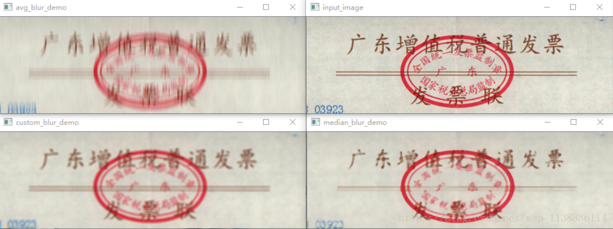
均值模糊（低通滤波）、中值模糊（中值滤波）

• 均值滤波：典型的线性滤波算法，它是指在图像上对目标像素给一个模板，该模板包括了其周围的临近像素（以目标像素为中心的周围8个像素，构成一个滤波模板，即去掉目标像素本身），再用模板中的全体像素的平均值来代替原来像素值。
• 中值滤波法是一种非线性平滑技术，它将每一像素点的灰度值设置为该点某邻域窗口内的所有像素点灰度值的中值。
   

import cv2
import numpy as np

# https://wangsp.blog.csdn.net/article/details/82872838

def blur_demo(image):            
	"""
	均值模糊 : 去随机噪声有很好的去噪效果
	（1, 15）是垂直方向模糊，（15， 1）是水平方向模糊
	"""
    dst = cv2.blur(image, (1, 15))    
    cv2.imshow("avg_blur_demo", dst)

def median_blur_demo(image):    # 中值模糊  对椒盐噪声有很好的去燥效果
    dst = cv2.medianBlur(image, 5)
    cv2.imshow("median_blur_demo", dst)

def custom_blur_demo(image):
	"""
	用户自定义模糊
	下面除以25是防止数值溢出
	"""
    kernel = np.ones([5, 5], np.float32)/25   
    dst = cv2.filter2D(image, -1, kernel)
    cv2.imshow("custom_blur_demo", dst)

src = cv2.imread("./fapiao.png")
img = cv2.resize(src,None,fx=0.8,fy=0.8,interpolation=cv2.INTER_CUBIC)
cv2.imshow('input_image', img)

blur_demo(img)
median_blur_demo(img)
custom_blur_demo(img)

cv2.waitKey(0)
cv2.destroyAllWindows()

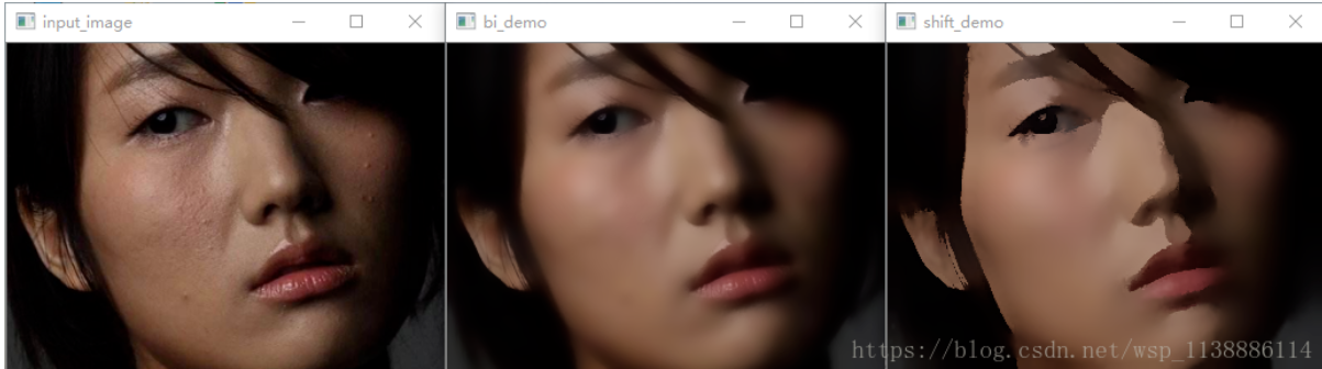
边缘保留滤波EPF

进行边缘保留滤波通常用到两个方法：高斯双边滤波和均值迁移滤波。

• 双边滤波（Bilateral filter）是一种非线性的滤波方法，是结合图像的空间邻近度和像素值相似度的一种折中处理，同时考虑空域信息和灰度相似性，达到保边去噪的目的。
• 双边滤波器顾名思义比高斯滤波多了一个高斯方差 σ－d，它是基于空间分布的高斯滤波函数，所以在边缘附近，离的较远的像素不会太多影响到边缘上的像素值，这样就保证了边缘附近像素值的保存。但是由于保存了过多的高频信息，对于彩色图像里的高频噪声，双边滤波器不能够干净的滤掉，只能够对于低频信息进行较好的滤波。
• 双边滤波函数原型：

"""
	bilateralFilter(src, d, sigmaColor, sigmaSpace[, dst[, borderType]]) -> dst
	  - src: 输入图像。
	  - d:   在过滤期间使用的每个像素邻域的直径。如果输入d非0，则sigmaSpace由d计算得出，如果sigmaColor没输入，则sigmaColor由sigmaSpace计算得出。
	  - sigmaColor: 色彩空间的标准方差，一般尽可能大。
	                较大的参数值意味着像素邻域内较远的颜色会混合在一起，
	                从而产生更大面积的半相等颜色。
	  - sigmaSpace: 坐标空间的标准方差(像素单位)，一般尽可能小。
	                参数值越大意味着只要它们的颜色足够接近，越远的像素都会相互影响。
	                当d > 0时，它指定邻域大小而不考虑sigmaSpace。 
	                否则，d与sigmaSpace成正比。
"""

import cv2

def bi_demo(image):      #双边滤波
    dst = cv2.bilateralFilter(image, 0, 100, 5)
    cv2.imshow("bi_demo", dst)

def shift_demo(image):   #均值迁移
    dst = cv2.pyrMeanShiftFiltering(image, 10, 50)
    cv2.imshow("shift_demo", dst)

src = cv2.imread('./100.png')
img = cv2.resize(src,None,fx=0.8,fy=0.8,
                 interpolation=cv2.INTER_CUBIC)
cv2.imshow('input_image', img)

bi_demo(img)
shift_demo(img)

cv2.waitKey(0)
cv2.destroyAllWindows()

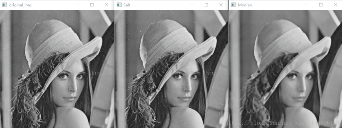
椒盐噪点（使用中值滤波去除）

import cv2
import numpy as np

def salt(img, n):
    for k in range(n):
        i = int(np.random.random() * img.shape[1])
        j = int(np.random.random() * img.shape[0])
        if img.ndim == 2:
            img[j,i] = 255
        elif img.ndim == 3:
            img[j,i,0]= 255
            img[j,i,1]= 255
            img[j,i,2]= 255
    return img

img = cv2.imread("./original_img.png",cv2.IMREAD_GRAYSCALE)
result = salt(img, 500)
median = cv2.medianBlur(result, 5)
cv2.imshow("original_img", img)
cv2.imshow("Salt", result)
cv2.imshow("Median", median)
cv2.waitKey(0)
cv2.destroyWindow()

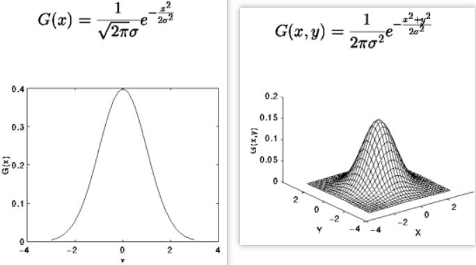
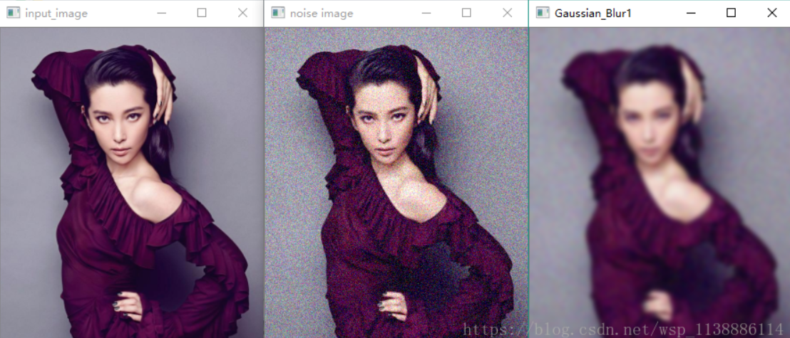
高斯滤波/模糊（去噪效果好）

• 高斯模糊实质上就是一种均值模糊，只是高斯模糊是按照加权平均的，距离越近的点权重越大，距离越远的点权重越小。
• 高斯滤波就是对整幅图像进行加权平均的过程，每一个像素点的值，都由其本身和邻域内的其他像素值经过加权平均后得到。

import cv2
import numpy as np

def clamp(pv):
    if pv > 255:
        return 255
    if pv < 0:
        return 0
    else:
        return pv

def gaussian_noise(image):           # 加高斯噪声
    h, w, c = image.shape
    for row in range(h):
        for col in range(w):
            s = np.random.normal(0, 20, 3)
            b = image[row, col, 0]   # blue
            g = image[row, col, 1]   # green
            r = image[row, col, 2]   # red
            image[row, col, 0] = clamp(b + s[0])
            image[row, col, 1] = clamp(g + s[1])
            image[row, col, 2] = clamp(r + s[2])
    cv2.imshow("noise image", image)

src = cv2.imread('888.png')
cv2.imshow('input_image', src)

gaussian_noise(src)
dst = cv2.GaussianBlur(src, (15,15), 0) #高斯模糊
cv2.imshow("Gaussian_Blur2", dst)

cv2.waitKey(0)
cv2.destroyAllWindows()

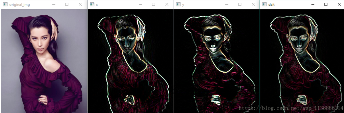
高通过滤/滤波（边缘检测/高反差保留）

使用的函数有：cv2.Sobel() , cv2.Schar() , cv2.Laplacian()
Sobel,scharr其实是求一阶或者二阶导数。scharr是对Sobel的优化。
Laplacian是求二阶导数。

• cv2.Sobel() 是一种带有方向过滤器

"""
dst = cv2.Sobel(src, ddepth, dx, dy[, dst[, ksize[, scale[, delta[, borderType]]]]])
src:    需要处理的图像；
ddepth: 图像的深度，-1表示采用的是与原图像相同的深度。 
        目标图像的深度必须大于等于原图像的深度；
dx和dy: 求导的阶数，0表示这个方向上没有求导，一般为0、1、2。

dst     不用解释了；
ksize： Sobel算子的大小，必须为1、3、5、7。  ksize=-1时，会用3x3的Scharr滤波器，
        它的效果要比3x3的Sobel滤波器要好 
scale： 是缩放导数的比例常数，默认没有伸缩系数；
delta： 是一个可选的增量，将会加到最终的dst中， 默认情况下没有额外的值加到dst中
borderType： 是判断图像边界的模式。这个参数默认值为cv2.BORDER_DEFAULT。

"""

import cv2

img=cv2.imread('888.png',cv2.IMREAD_COLOR)
x=cv2.Sobel(img,cv2.CV_16S,1,0)
y=cv2.Sobel(img,cv2.CV_16S,0,1)

absx=cv2.convertScaleAbs(x)
absy=cv2.convertScaleAbs(y)
dist=cv2.addWeighted(absx,0.5,absy,0.5,0)

cv2.imshow('original_img',img)
cv2.imshow('y',absy)
cv2.imshow('x',absx)
cv2.imshow('dsit',dist)

cv2.waitKey(0)
cv2.destroyAllWindows()

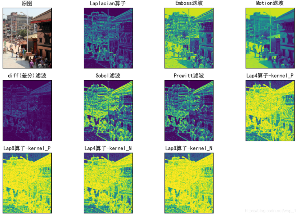
其它滤波（Emboss,Motion,different,Sobel,Prewitt,LoG）

import matplotlib.pyplot as plt
import numpy as np
import cv2


def log_filter(gray_img):
    gaus_img = cv2.GaussianBlur(gray_img,(3,3),sigmaX=0)  # 以核大小为3x3，方差为0
    log_img = cv2.Laplacian(gaus_img,cv2.CV_16S,ksize=3)  # laplace检测
    log_img = cv2.convertScaleAbs(log_img)
    return log_img


def filter_imgs(gray_img):
    # 尝试一下不同的核的效果
    Emboss = np.array([[ -2,-1, 0],
                       [ -1, 1, 1],
                       [  0, 1, 2]])

    Motion = np.array([[ 0.333, 0,  0],
                       [  0, 0.333, 0],
                       [  0, 0, 0.333]])

    Emboss_img = cv2.filter2D(gray_img,cv2.CV_16S,Emboss)
    Motion_img = cv2.filter2D(gray_img, cv2.CV_16S, Motion)
    Emboss_img = cv2.convertScaleAbs(Emboss_img)
    Motion_img = cv2.convertScaleAbs(Motion_img)

    different_V = np.array([[  0, -1, 0],
                            [  0,  1, 0],
                            [  0,  0, 0]])
    different_H = np.array([[  0, 0, 0],
                            [ -1, 1, 0],
                            [  0, 0, 0]])
    different_temp = cv2.filter2D(gray_img,cv2.CV_16S,different_V)
    different_temp = cv2.filter2D(different_temp, cv2.CV_16S, different_H)
    different_img = cv2.convertScaleAbs(different_temp)

    Sobel_V = np.array([[ 1,  2,  1],
                        [ 0,  0,  0],
                        [ -1, -2, -1]])
    Sobel_H = np.array([[ 1,  0, -1],
                        [ 2,  0, -2],
                        [ 1,  0, -1]])
    Sobel_temp = cv2.filter2D(gray_img,cv2.CV_16S, Sobel_V)
    Sobel_temp = cv2.filter2D(Sobel_temp, cv2.CV_16S, Sobel_H)
    Sobel_img = cv2.convertScaleAbs(Sobel_temp)


    Prewitt_V = np.array([[-1, -1, -1],
                          [ 0,  0,  0],
                          [ 1,  1,  1]])
    Prewitt_H = np.array([[-1,  0, 1],
                          [-1,  0, 1],
                          [-1,  0, 1]])
    Prewitt_temp = cv2.filter2D(gray_img, cv2.CV_16S, Prewitt_V)
    Prewitt_temp = cv2.filter2D(Prewitt_temp, cv2.CV_16S, Prewitt_H)
    Prewitt_img = cv2.convertScaleAbs(Prewitt_temp)

    kernel_P = np.array([[0,  0, -1,  0, 0],
                         [0, -1, -2, -1, 0],
                         [-1,-2, 16, -2,-1],
                         [0, -1, -2, -1, 0],
                         [0, 0,  -1, 0,  0]])
    kernel_N = np.array([[0, 0,  1,  0, 0],
                         [0, 1,  2,  1, 0],
                         [1, 2, -16, 2, 1],
                         [0, 1,  2,  1, 0],
                         [0, 0,  1,  0, 0]])


    lap4_filter = np.array([[0, 1, 0],
                            [1, -4, 1],
                            [0, 1, 0]])  # 4邻域laplacian算子
    lap8_filter = np.array([[0, 1, 0],
                            [1, -8, 1],
                            [0, 1, 0]])  # 8邻域laplacian算子
    lap_filter_P = cv2.filter2D(gray_img, cv2.CV_16S, kernel_P)
    edge4_img_P = cv2.filter2D(lap_filter_P, cv2.CV_16S, lap4_filter)
    edge4_img_P = cv2.convertScaleAbs(edge4_img_P)

    edge8_img_P = cv2.filter2D(lap_filter_P, cv2.CV_16S, lap8_filter)
    edge8_img_P = cv2.convertScaleAbs(edge8_img_P)


    lap_filter_N = cv2.filter2D(gray_img, cv2.CV_16S, kernel_N)
    edge4_img_N = cv2.filter2D(lap_filter_N, cv2.CV_16S, lap4_filter)
    edge4_img_N = cv2.convertScaleAbs(edge4_img_N)

    edge8_img_N = cv2.filter2D(lap_filter_N, cv2.CV_16S, lap8_filter)
    edge8_img_N = cv2.convertScaleAbs(edge8_img_N)
    return (Emboss_img,Motion_img,different_img,Sobel_img,Prewitt_img,edge4_img_P,edge8_img_P,edge4_img_N,edge8_img_N)




def show(Filter_imgs):
    titles = [u'原图',     u'Laplacian算子',\
              u'Emboss滤波',u'Motion滤波',
              u'diff(差分)滤波',u'Sobel滤波',u'Prewitt滤波',
              u'Lap4算子-kernel_P', u'Lap8算子-kernel_P',
              u'Lap4算子-kernel_N', u'Lap8算子-kernel_N']

    plt.rcParams['font.sans-serif'] = ['SimHei']
    plt.figure(figsize=(12, 8))
    for i in range(len(titles)):
        plt.subplot(3, 4, i + 1)
        plt.imshow(Filter_imgs[i])
        plt.title(titles[i])
        plt.xticks([]), plt.yticks([])
    plt.show()


if __name__ == '__main__':
    img = cv2.imread('yinying3.png')
    img_raw   = cv2.cvtColor(img, cv2.COLOR_BGR2RGB)
    gray_img = cv2.cvtColor(img, cv2.COLOR_BGR2GRAY)

    LoG_img = log_filter(gray_img)
    Filter_imgs = [img_raw,LoG_img]
    Filter_imgs.extend(filter_imgs(gray_img))
    show(Filter_imgs)

参考博客

Pytorch 实现sobel算子的卷积操作_洪流之源的博客-CSDN博客_卷积实现sobel

（七）滤波与卷积_淡定的炮仗的博客-CSDN博客_卷积滤波

图像处理之高通滤波及低通滤波_ReWz的博客-CSDN博客_低通滤波和高通滤波对图像的影响

数字图像处理——图像梯度和空间滤波 - 知乎 (zhihu.com)

OpenCV—Python 图像滤波（均值、中值、高斯、高斯双边、高通等滤波）_SongpingWang的博客-CSDN博客