如何用python做数据分析

最近，Analysis with Programming加入了Planet Python。我这里来分享一下如何通过Python来开始数据分析。具体内容如下：

数据导入

导入本地的或者web端的CSV文件；

数据变换；

数据统计描述；

假设检验

单样本t检验；

可视化；

创建自定义函数。

数据导入

1. 1

   这是很关键的一步，为了后续的分析我们首先需要导入数据。通常来说，数据是CSV格式，就算不是，至少也可以转换成CSV格式。在Python中，我们的操作如下：

   import pandas as pd

   # Reading data locally

   df = pd.read_csv('/Users/al-ahmadgaidasaad/Documents/d.csv')

   # Reading data from web

   data_url = "https://raw.githubusercontent.com/alstat/Analysis-with-Programming/master/2014/Python/Numerical-Descriptions-of-the-Data/data.csv"

   df = pd.read_csv(data_url)

   为了读取本地CSV文件，我们需要pandas这个数据分析库中的相应模块。其中的read_csv函数能够读取本地和web数据。

   END

数据变换

1. 1

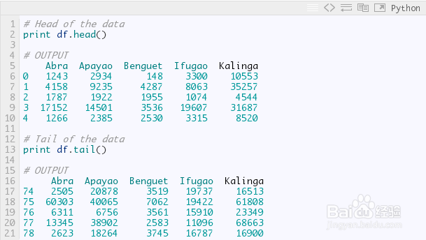
   既然在工作空间有了数据，接下来就是数据变换。统计学家和科学家们通常会在这一步移除分析中的非必要数据。我们先看看数据（下图）

   对R语言程序员来说，上述操作等价于通过print(head(df))来打印数据的前6行，以及通过print(tail(df))来打印数据的后6行。当然Python中，默认打印是5行，而R则是6行。因此R的代码head(df, n = 10)，在Python中就是df.head(n = 10)，打印数据尾部也是同样道理

   

2. 2

   在R语言中，数据列和行的名字通过colnames和rownames来分别进行提取。在Python中，我们则使用columns和index属性来提取，如下：

   # Extracting column names

   print df.columns

   # OUTPUT

   Index([u'Abra', u'Apayao', u'Benguet', u'Ifugao', u'Kalinga'], dtype='object')

   # Extracting row names or the index

   print df.index

   # OUTPUT

   Int64Index([0, 1, 2, 3, 4, 5, 6, 7, 8, 9, 10, 11, 12, 13, 14, 15, 16, 17, 18, 19, 20, 21, 22, 23, 24, 25, 26, 27, 28, 29, 30, 31, 32, 33, 34, 35, 36, 37, 38, 39, 40, 41, 42, 43, 44, 45, 46, 47, 48, 49, 50, 51, 52, 53, 54, 55, 56, 57, 58, 59, 60, 61, 62, 63, 64, 65, 66, 67, 68, 69, 70, 71, 72, 73, 74, 75, 76, 77, 78], dtype='int64')

3. 3

   数据转置使用T方法，

   # Transpose data

   print df.T

   # OUTPUT

               0      1     2      3     4      5     6      7     8      9   

   Abra      1243   4158  1787  17152  1266   5576   927  21540  1039   5424   

   Apayao    2934   9235  1922  14501  2385   7452  1099  17038  1382  10588   

   Benguet    148   4287  1955   3536  2530    771  2796   2463  2592   1064   

   Ifugao    3300   8063  1074  19607  3315  13134  5134  14226  6842  13828   

   Kalinga  10553  35257  4544  31687  8520  28252  3106  36238  4973  40140   

            ...       69     70     71     72     73     74     75     76     77  

   Abra     ...    12763   2470  59094   6209  13316   2505  60303   6311  13345   

   Apayao   ...    37625  19532  35126   6335  38613  20878  40065   6756  38902   

   Benguet  ...     2354   4045   5987   3530   2585   3519   7062   3561   2583   

   Ifugao   ...     9838  17125  18940  15560   7746  19737  19422  15910  11096   

   Kalinga  ...    65782  15279  52437  24385  66148  16513  61808  23349  68663   

               78  

   Abra      2623  

   Apayao   18264  

   Benguet   3745  

   Ifugao   16787  

   Kalinga  16900  

   Other transformations such as sort can be done using <code>sort</code> attribute. Now let's extract a specific column. In Python, we do it using either <code>iloc</code> or <code>ix</code> attributes, but <code>ix</code> is more robust and thus I prefer it. Assuming we want the head of the first column of the data, we have

4. 4

   其他变换，例如排序就是用sort属性。现在我们提取特定的某列数据。Python中，可以使用iloc或者ix属性。但是我更喜欢用ix，因为它更稳定一些。假设我们需数据第一列的前5行，我们有：

   print df.ix[:, 0].head()   

   # OUTPUT 0     1243 1     4158 2     1787 3    17152 4     1266 Name: Abra, dtype: int64

5. 5

   顺便提一下，Python的索引是从0开始而非1。为了取出从11到20行的前3列数据，我们有

   print df.ix[10:20, 0:3]

   # OUTPUT

       Abra  Apayao  Benguet

   10    981    1311     2560

   11  27366   15093     3039

   12   1100    1701     2382

   13   7212   11001     1088

   14   1048    1427     2847

   15  25679   15661     2942

   16   1055    2191     2119

   17   5437    6461      734

   18   1029    1183     2302

   19  23710   12222     2598

   20   1091    2343     2654

   上述命令相当于df.ix[10:20, ['Abra', 'Apayao', 'Benguet']]。

6. 6

   为了舍弃数据中的列，这里是列1(Apayao)和列2(Benguet)，我们使用drop属性，如下：

   print df.drop(df.columns[[1, 2]], axis = 1).head()

   # OUTPUT

       Abra  Ifugao  Kalinga

   0   1243    3300    10553

   1   4158    8063    35257

   2   1787    1074     4544

   3  17152   19607    31687

   4   1266    3315     8520

   axis 参数告诉函数到底舍弃列还是行。如果axis等于0，那么就舍弃行。

   END

统计描述

1. 1

   下一步就是通过describe属性，对数据的统计特性进行描述：

   print df.describe()

   # OUTPUT

                  Abra        Apayao      Benguet        Ifugao       Kalinga

   count     79.000000     79.000000    79.000000     79.000000     79.000000

   mean   12874.379747  16860.645570  3237.392405  12414.620253  30446.417722

   std    16746.466945  15448.153794  1588.536429   5034.282019  22245.707692

   min      927.000000    401.000000   148.000000   1074.000000   2346.000000

   25%     1524.000000   3435.500000  2328.000000   8205.000000   8601.500000

   50%     5790.000000  10588.000000  3202.000000  13044.000000  24494.000000

   75%    13330.500000  33289.000000  3918.500000  16099.500000  52510.500000

   max    60303.000000  54625.000000  8813.000000  21031.000000  68663.000000

   END

假设检验

1. 1

   Python有一个很好的统计推断包。那就是scipy里面的stats。ttest_1samp实现了单样本t检验。因此，如果我们想检验数据Abra列的稻谷产量均值，通过零假设，这里我们假定总体稻谷产量均值为15000，我们有：

   from scipy import stats as ss

   # Perform one sample t-test using 1500 as the true mean

   print ss.ttest_1samp(a = df.ix[:, 'Abra'], popmean = 15000)

   # OUTPUT

   (-1.1281738488299586, 0.26270472069109496)

   返回下述值组成的元祖：

   t : 浮点或数组类型t统计量

   prob : 浮点或数组类型two-tailed p-value 双侧概率值

2. 2

   通过上面的输出，看到p值是0.267远大于α等于0.05，因此没有充分的证据说平均稻谷产量不是150000。将这个检验应用到所有的变量，同样假设均值为15000，我们有：

   print ss.ttest_1samp(a = df, popmean = 15000)

   # OUTPUT

   (array([ -1.12817385,   1.07053437, -65.81425599,  -4.564575  ,   6.17156198]),

    array([  2.62704721e-01,   2.87680340e-01,   4.15643528e-70,

             1.83764399e-05,   2.82461897e-08]))

   第一个数组是t统计量，第二个数组则是相应的p值

   END

可视化

1. 1

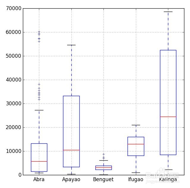
   Python中有许多可视化模块，最流行的当属matpalotlib库。稍加提及，我们也可选择bokeh和seaborn模块。之前的博文中，我已经说明了matplotlib库中的盒须图模块功能。

   

2. 2

   # Import the module for plotting

   import matplotlib.pyplot as plt

    plt.show(df.plot(kind = 'box'))

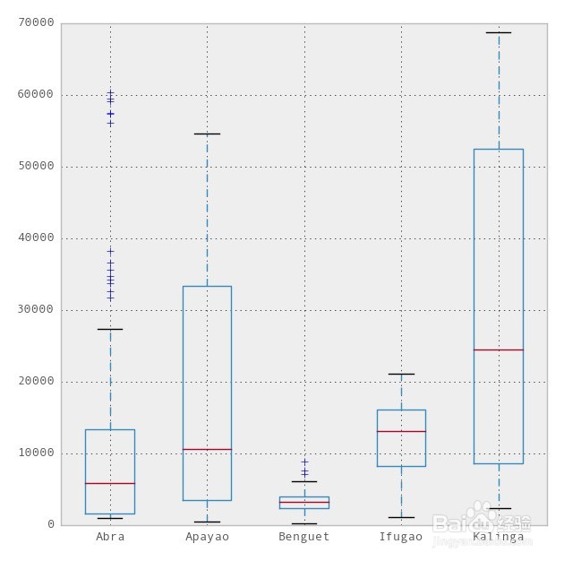
   现在，我们可以用pandas模块中集成R的ggplot主题来美化图表。要使用ggplot，我们只需要在上述代码中多加一行，

   import matplotlib.pyplot as plt

   pd.options.display.mpl_style = 'default' # Sets the plotting display theme to ggplot2

   df.plot(kind = 'box')

3. 这样我们就得到如下图表：

   

4. 比matplotlib.pyplot主题简洁太多。但是在本文中，我更愿意引入seaborn模块，该模块是一个统计数据可视化库。因此我们有：

   # Import the seaborn library

   import seaborn as sns

    # Do the boxplot

   plt.show(sns.boxplot(df, widths = 0.5, color = "pastel"))

   

5. 多性感的盒式图，继续往下看。

   

6. plt.show(sns.violinplot(df, widths = 0.5, color = "pastel"))

   

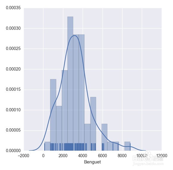
7. plt.show(sns.distplot(df.ix[:,2], rug = True, bins = 15))

   

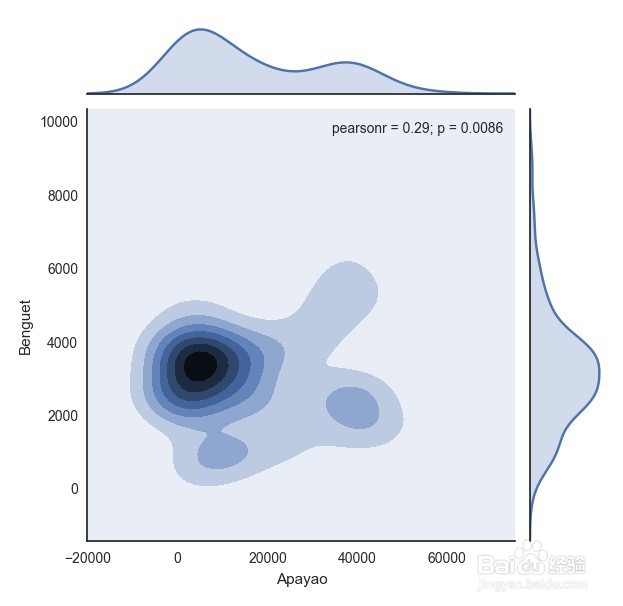
8. with sns.axes_style("white"):

       plt.show(sns.jointplot(df.ix[:,1], df.ix[:,2], kind = "kde"))

   

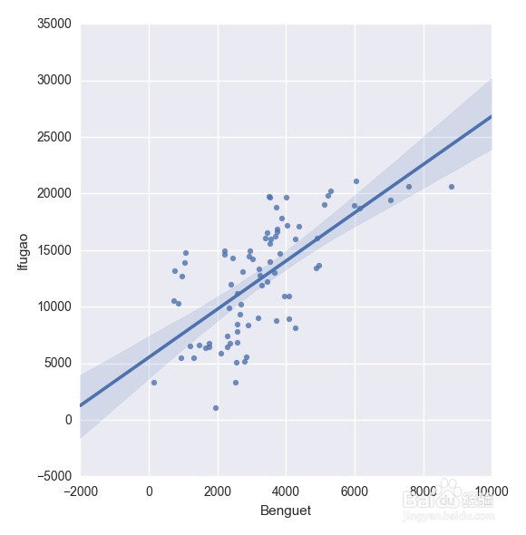
9. plt.show(sns.lmplot("Benguet", "Ifugao", df))

   END

创建自定义函数

1. 在Python中，我们使用def函数来实现一个自定义函数。例如，如果我们要定义一个两数相加的函数，如下即可：

   def add_2int(x, y):

       return x + y

   print add_2int(2, 2)

   # OUTPUT

   4

2. 顺便说一下，Python中的缩进是很重要的。通过缩进来定义函数作用域，就像在R语言中使用大括号{…}一样。这有一个我们之前博文的例子：

   产生10个正态分布样本，其中和

   基于95%的置信度，计算和 ;

   重复100次; 然后

   计算出置信区间包含真实均值的百分比

   Python中，程序如下：

   import numpy as np

   import scipy.stats as ss

   def case(n = 10, mu = 3, sigma = np.sqrt(5), p = 0.025, rep = 100):

       m = np.zeros((rep, 4))

       for i in range(rep):

           norm = np.random.normal(loc = mu, scale = sigma, size = n)

           xbar = np.mean(norm)

           low = xbar - ss.norm.ppf(q = 1 - p) * (sigma / np.sqrt(n))

           up = xbar + ss.norm.ppf(q = 1 - p) * (sigma / np.sqrt(n))

           if (mu > low) & (mu < up):

               rem = 1

           else:

               rem = 0

           m[i, :] = [xbar, low, up, rem]

       inside = np.sum(m[:, 3])

       per = inside / rep

       desc = "There are " + str(inside) + " confidence intervals that contain " 

              "the true mean (" + str(mu) + "), that is " + str(per) + " percent of the total CIs"

       return {"Matrix": m, "Decision": desc}

3. 上述代码读起来很简单，但是循环的时候就很慢了。下面针对上述代码进行了改进，这多亏了 Python专家

   import numpy as np

   import scipy.stats as ss

   def case2(n = 10, mu = 3, sigma = np.sqrt(5), p = 0.025, rep = 100):

       scaled_crit = ss.norm.ppf(q = 1 - p) * (sigma / np.sqrt(n))

       norm = np.random.normal(loc = mu, scale = sigma, size = (rep, n))

       xbar = norm.mean(1)

       low = xbar - scaled_crit

       up = xbar + scaled_crit

       rem = (mu > low) & (mu < up)

       m = np.c_[xbar, low, up, rem]

       inside = np.sum(m[:, 3])

       per = inside / rep

       desc = "There are " + str(inside) + " confidence intervals that contain " 

              "the true mean (" + str(mu) + "), that is " + str(per) + " percent of the total CIs"

       return {"Matrix": m, "Decision": desc}

知道你对python感兴趣，所以给你准备了下面的资料~

 这份完整版的Python全套学习资料已经上传，朋友们如果需要可以点击链接免费领取或者滑到最后扫描二v码【保证100%免费】

python学习资源免费分享，保证100%免费！！！

需要的话可以点击这里👉Python学习路线（2023修正版）附涉及资料 （安全链接，放心点击）

文末有福利领取哦~ 

一、Python所有方向的学习路线

Python所有方向的技术点做的整理，形成各个领域的知识点汇总，它的用处就在于，你可以按照上面的知识点去找对应的学习资源，保证自己学得较为全面。​​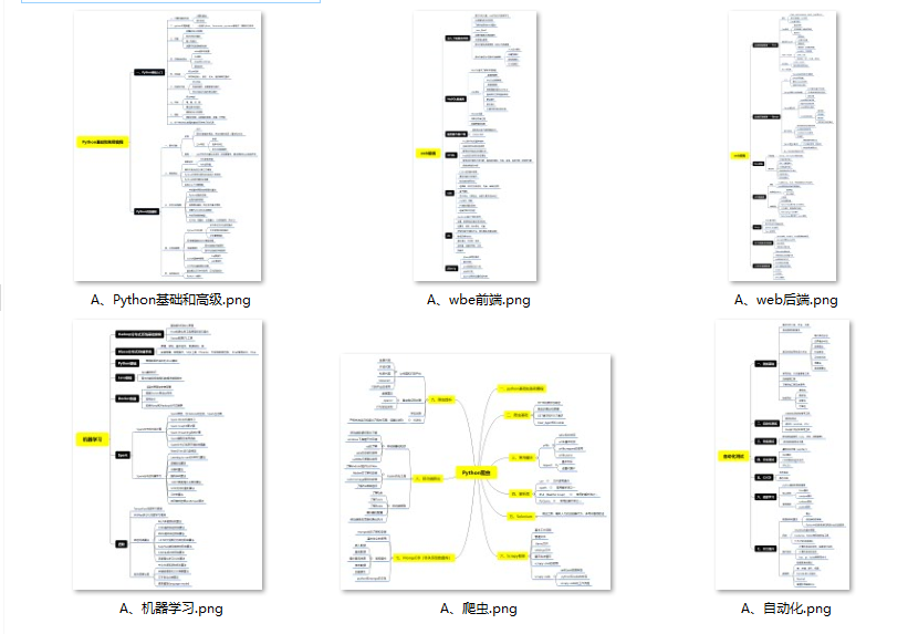

二、Python必备开发工具

​​

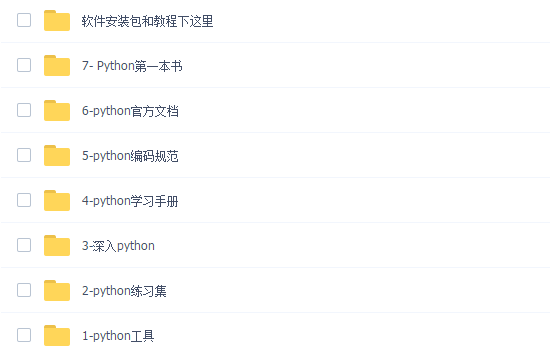
三、精品Python学习书籍

当我学到一定基础，有自己的理解能力的时候，会去阅读一些前辈整理的书籍或者手写的笔记资料，这些笔记详细记载了他们对一些技术点的理解，这些理解是比较独到，可以学到不一样的思路。
​​

四、Python视频合集

观看零基础学习视频，看视频学习是最快捷也是最有效果的方式，跟着视频中老师的思路，从基础到深入，还是很容易入门的。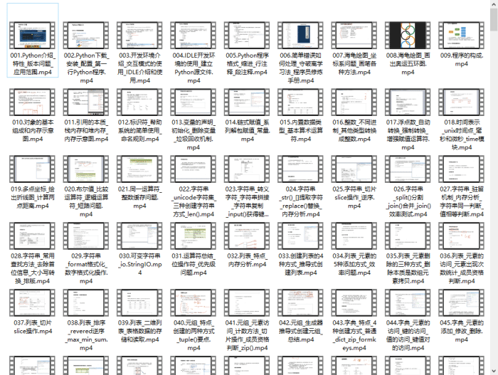
​​
​​

五、实战案例

光学理论是没用的，要学会跟着一起敲，要动手实操，才能将自己的所学运用到实际当中去，这时候可以搞点实战案例来学习。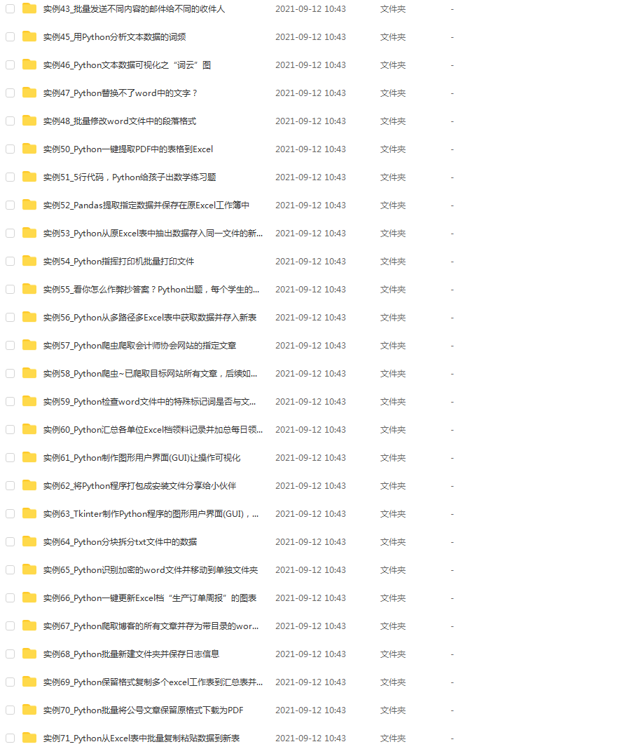
​​

六、Python练习题

检查学习结果。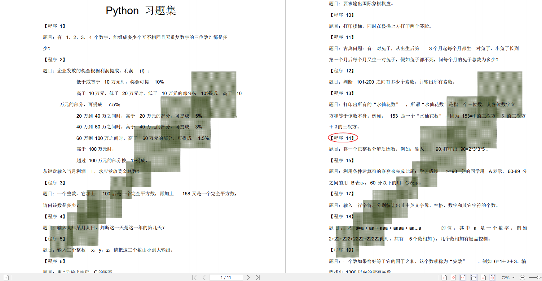
​​

七、面试资料

我们学习Python必然是为了找到高薪的工作，下面这些面试题是来自阿里、腾讯、字节等一线互联网大厂最新的面试资料，并且有阿里大佬给出了权威的解答，刷完这一套面试资料相信大家都能找到满意的工作。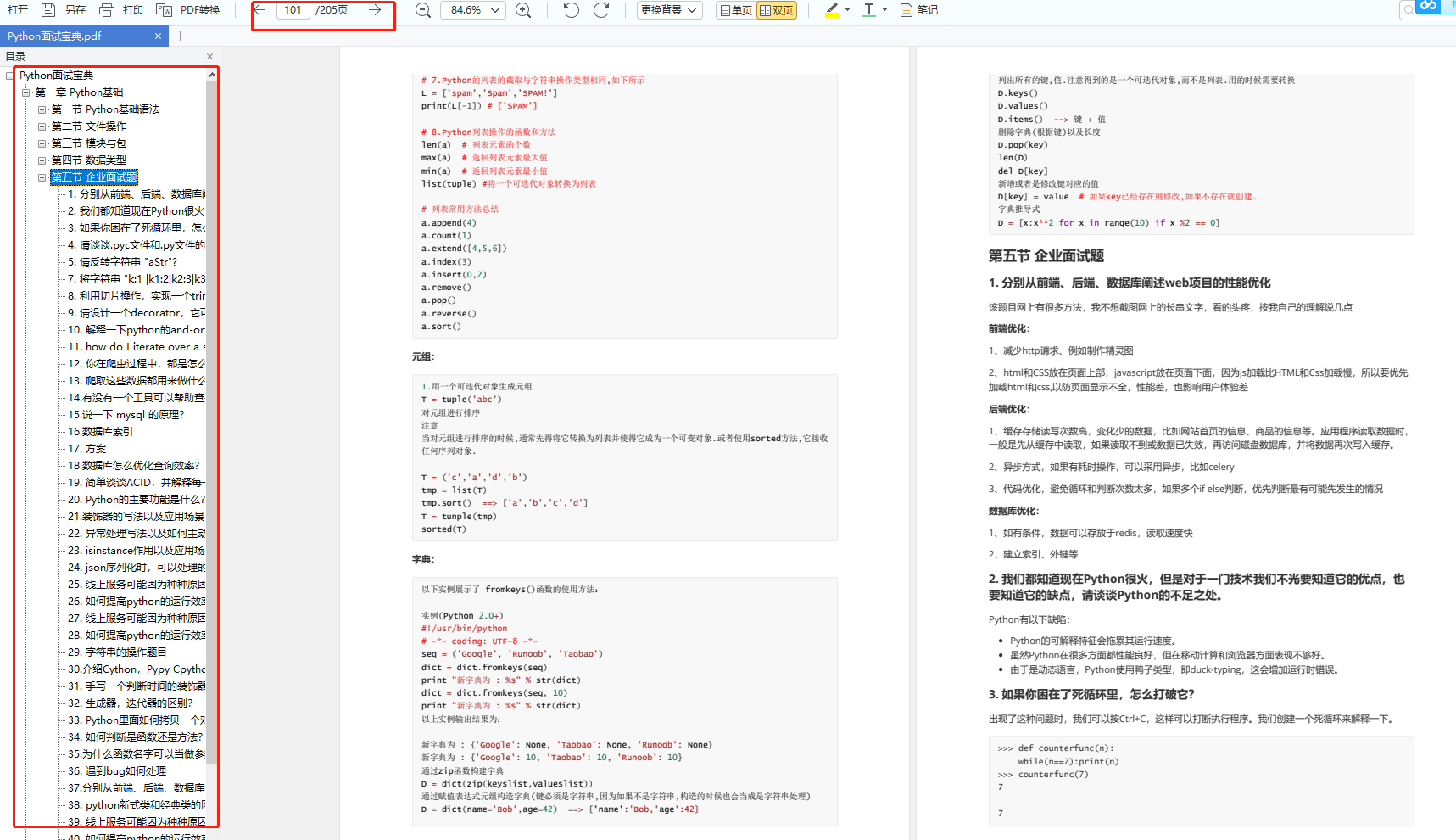
​​
​​

 👉这份完整版的Python全套学习资料已经上传，朋友们如果需要可以扫描下方CSDN官方认证二维码或者点击链接免费领取【保证100%免费】
Python学习路线（2023修正版）附涉及资料《Python学习资料》，已经打包好了，自取【ps：需要领取的资料（请备注清楚，查找与发送给你）】。因链接常https://mp.weixin.qq.com/s/UVxw0daFCgAMFhz9cfrjAQ