paper and paper：GitHub - clovaai/stargan-v2: StarGAN v2 - Official PyTorch Implementation (CVPR 2020)

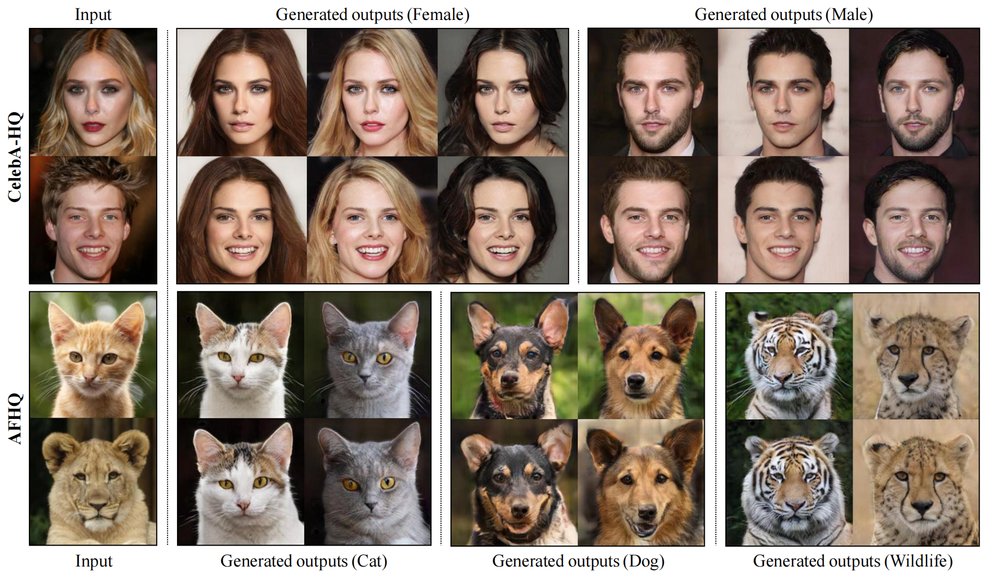
 Figure 1. The first column shows input images while the remaining columns are images synthesized by StarGAN v2.

摘要

优秀的图像-图像转换模型需要学习不同视觉域之间的映射，要同时满足以下属性：1）生成图像的多样性    2）在多个域上的可扩展性。因此提出了star-GAN v2和动物数据集AFHQ

一.介绍

域：可以分组为视觉上独特的类别的不同组图片（比如，可以根据性别将人分为男性和女性两个域）
风格：每组图片中的每张图片都有独特的外观，这称之为风格。（而人物的装扮，胡子，发型等特征可以视为风格）
大概就是范围更大的可区分特征叫做域，范围小的叫做风格，一个理想的图像转换模型应该考虑域内的多样化的风格。但这种模型的设计和学习很困难，因为一种域内可以有大量的任意风格。

为了实现风格多样性：将从标准高斯分布中随机采样的低维隐向量喂给生成器，然后不同域的解码器则从上述向量中取得自己所需的风格内容，然后生成图片，这种一对一的映射会导致实现风格的多样性需要多种生成器，如K域，则需要K(K-1)个生成器。

为了实现可扩展性。star gan通过将输入图片于特定的域标签级联，使用一个生成器实现将输入图片转换到目标域的图片，但是这只是学到了每个域的确定映射（给标签的那一刻就确定了，毕竟是只给了一个one hot的标签），不能学到数据分布多种模态的特性（相当于不能同时转换多种风格）。因此，如果使用风格特征代替域标签，那么引入的信息会更多。

改进1：将star gan中的域标签用特定域的风格特征（不是单一风格，如这个风格特征保护胡须，发型，性别等风格）代替，实现风格的多样性。使用了风格编码网络（提取目标图片的风格）和maping net（随机高斯噪声转换成目标域的一种随机的风格特征）来实现。当有多个域的时候，每个模块都将有多个输出分支，每个分支表示特定域的风格特征

二.StarGANv2

给出图片x和任意一个目标域的图片y，生成具有x的内容但是包含y的风格的图片。

1.网络结构

StarGAN 改进版本，不需要具体标出style标签（attribute），只需：

1、输入源domain的图像，以及目标domain的一张指定参考图像（Style Encoder网络学习其style code），就可将源图像转换成 目标domain+参考图像style 的迁移图像；或者
2、输入源domain的图像，以及随机噪声(mapping网络将其映射为指定domain的随机style code)，就可将源图像转换成 目标domain+随机style 的迁移图像
Stargan v2 结构如下：

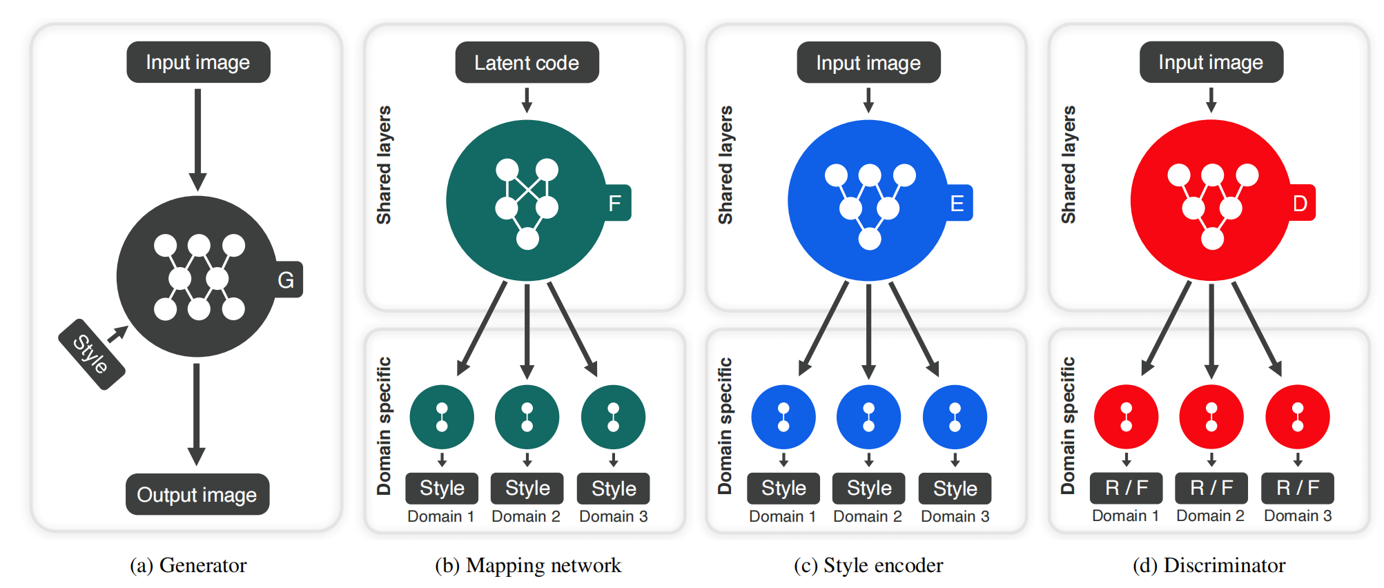
Figure 2.  consisting of four modules.
(a) The generator translates an input image into an output image reflecting the domain-specific style code.
(b) The mapping network transforms a latent code into style codes for multiple domains, one of which is randomly selected during training.
(c) The style encoder extracts the style code of an image, allowing the generator to perform reference guided image synthesis.
(d) The discriminator distinguishes between real and fake images from multiple domains.

Note that all modules except the generator contain multiple output branches, one of which is selected when training the corresponding domain.

生成器：

生成器G（x，s）需要输入图像x和特定风格编码s，s由Mapping network F或者Style encoder E提供。我们使用adaptive instance normalization（AdaIN）变换，而不是直接级联来将s注入到G中，从而生成一张具有s风格的图片。
 

Mapping net：

给定一个潜在编码z和一个域y，映射网络F生成风格编码，其中表示F对应于域y的输出。F由带有多个输出分支的MLP组成，用来为所有可用域提供风格编码。F 通过随机采样潜在向量z和域y来提供多样化风格编码。我们的多任务架构允许F高效地学习所有域的风格表达。

将一个隐向量z映射到不同域的风格特征，相当于mappingNet是一个多任务的全连接网络。训练的时候是随机采样Z中的样本z和随机采样域Y中的一张图片来使得该网络有效的学到所有域的风格表示。感觉有点像VAE?变换个参数（这里是稍微改变z），就可以得到目标域的风格相似的特征，因此可以实现多样性风格生成。

Style encoder：

给定图像x和它对应的域y，编码器E提取风格编码. 其中  表示编码器特定域域y的输出。和F类似，风格编码器E也受益于多任务学习设置。E可以使用不同参考图片生成多样化风格编码。这允许G合成反映参考图像x的风格s的输出图像。

使用一个多任务的风格特征提取网络。因此，使用不同的参考图片训练，该网络可以提供多样性的风格特征。

判别器：
多任务分类器，有多个输出分支。每个分支使用一个二进制分类判断真实图片x是否真实以及生成图片是否则真实。使用多个分类器是为了避免笼统地判断生成地是否真实，因为我们要的是生成地图片在特定域上地真实，而不是随便地真实，优化更加具体了。

改进过程如下表：

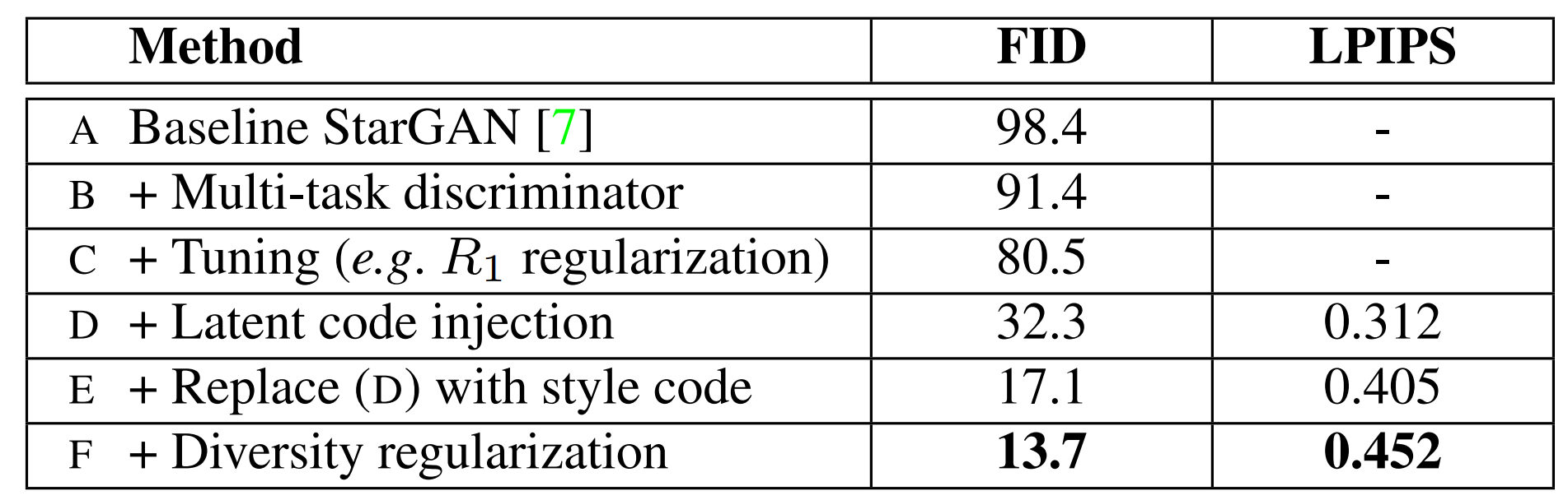
 Table 1. Frechet inception distance (FID) indicates the distance between two distributions of real and generated images (lower is better), while learned perceptual image patch similarity (LPIPS) measures the diversity of generated images (higher is better).

基于（A）StarGAN，改进尝试如下，每点改进效果见下图：

• （B）将原ACGAN+PatchGAN的鉴别器 换成 多任务鉴别器，使生成器能转换全局结构。
• （C）引入R1正则与AdIN增加稳定度
• （D）直接引入潜变量z增加多样性（无法有效，只能改变某一固定区域，而不是全局）
• （E）将(D)的改进换成 引入映射网络，输出为每个domain的style code
• （F）多样性正则

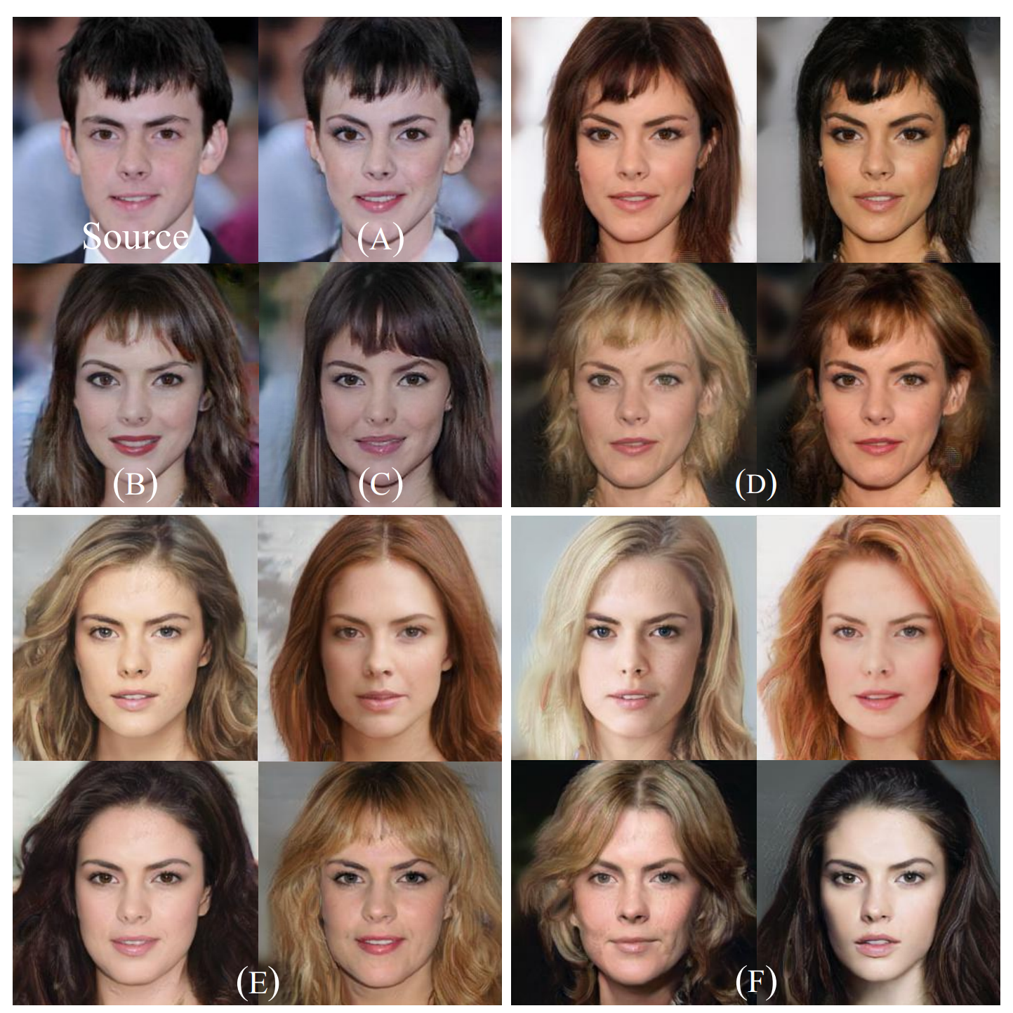
 Figure 3. Note that given a source image, the configurations (A) - (C) provide a single output, while (D) - (F) generate multiple output images.

2、具体结构

①、Generator

对AFHQ数据集如下，4个下采样块，4个中间块以及4个上采样块，如下表所示。对CelebA HQ，下采样以及上采样块数加一。

 其结构图如下：

 

 其代码如下：

class Generator(nn.Module):
    def __init__(self, img_size=256, style_dim=64, max_conv_dim=512, w_hpf=1):
        super().__init__()
        dim_in = 2**14 // img_size
        self.img_size = img_size
        self.from_rgb = nn.Conv2d(3, dim_in, 3, 1, 1)
        self.encode = nn.ModuleList()
        self.decode = nn.ModuleList()
        self.to_rgb = nn.Sequential(
            nn.InstanceNorm2d(dim_in, affine=True),
            nn.LeakyReLU(0.2),
            nn.Conv2d(dim_in, 3, 1, 1, 0))

        # down/up-sampling blocks
        repeat_num = int(np.log2(img_size)) - 4
        if w_hpf > 0: #weight for high-pass filtering
            repeat_num += 1
        for _ in range(repeat_num):
            dim_out = min(dim_in*2, max_conv_dim)
            self.encode.append(
                ResBlk(dim_in, dim_out, normalize=True, downsample=True))
            self.decode.insert(
                0, AdainResBlk(dim_out, dim_in, style_dim,
                               w_hpf=w_hpf, upsample=True))  # stack-like
            dim_in = dim_out

        # bottleneck blocks
        for _ in range(2):
            self.encode.append(
                ResBlk(dim_out, dim_out, normalize=True))
            self.decode.insert(
                0, AdainResBlk(dim_out, dim_out, style_dim, w_hpf=w_hpf))

        if w_hpf > 0:
            device = torch.device(
                'cuda' if torch.cuda.is_available() else 'cpu')
            self.hpf = HighPass(w_hpf, device)

    def forward(self, x, s, masks=None):
        x = self.from_rgb(x)
        cache = {}
        for block in self.encode:
            if (masks is not None) and (x.size(2) in [32, 64, 128]):
                cache[x.size(2)] = x
            x = block(x)
        for block in self.decode:
            x = block(x, s)
            if (masks is not None) and (x.size(2) in [32, 64, 128]):
                mask = masks[0] if x.size(2) in [32] else masks[1]
                mask = F.interpolate(mask, size=x.size(2), mode='bilinear')
                x = x + self.hpf(mask * cache[x.size(2)])
        return self.to_rgb(x)
        
class AdaIN(nn.Module):
    def __init__(self, style_dim, num_features):
        super().__init__()
        self.norm = nn.InstanceNorm2d(num_features, affine=False)
        self.fc = nn.Linear(style_dim, num_features*2)

    def forward(self, x, s):
        h = self.fc(s)
        h = h.view(h.size(0), h.size(1), 1, 1)
        gamma, beta = torch.chunk(h, chunks=2, dim=1) ## 分成两块
        return (1 + gamma) * self.norm(x) + beta       
        
class ResBlk(nn.Module):
    def __init__(self, dim_in, dim_out, actv=nn.LeakyReLU(0.2),
                 normalize=False, downsample=False):
        super().__init__()
        self.actv = actv
        self.normalize = normalize
        self.downsample = downsample
        self.learned_sc = dim_in != dim_out
        self._build_weights(dim_in, dim_out)

    def _build_weights(self, dim_in, dim_out):
        self.conv1 = nn.Conv2d(dim_in, dim_in, 3, 1, 1)
        self.conv2 = nn.Conv2d(dim_in, dim_out, 3, 1, 1)
        if self.normalize:
            self.norm1 = nn.InstanceNorm2d(dim_in, affine=True)
            self.norm2 = nn.InstanceNorm2d(dim_in, affine=True)
        if self.learned_sc:
            self.conv1x1 = nn.Conv2d(dim_in, dim_out, 1, 1, 0, bias=False)

    def _shortcut(self, x):
        if self.learned_sc:
            x = self.conv1x1(x)
        if self.downsample:
            x = F.avg_pool2d(x, 2)
        return x

    def _residual(self, x):
        if self.normalize:
            x = self.norm1(x)
        x = self.actv(x)
        x = self.conv1(x)
        if self.downsample:
            x = F.avg_pool2d(x, 2)
        if self.normalize:
            x = self.norm2(x)
        x = self.actv(x)
        x = self.conv2(x)
        return x

    def forward(self, x):
        x = self._shortcut(x) + self._residual(x)
        return x / math.sqrt(2)  # unit variance ***

class AdainResBlk(nn.Module):
    def __init__(self, dim_in, dim_out, style_dim=64, w_hpf=0,
                 actv=nn.LeakyReLU(0.2), upsample=False):
        super().__init__()
        self.w_hpf = w_hpf
        self.actv = actv
        self.upsample = upsample
        self.learned_sc = dim_in != dim_out
        self._build_weights(dim_in, dim_out, style_dim)

    def _build_weights(self, dim_in, dim_out, style_dim=64):
        self.conv1 = nn.Conv2d(dim_in, dim_out, 3, 1, 1)
        self.conv2 = nn.Conv2d(dim_out, dim_out, 3, 1, 1)
        self.norm1 = AdaIN(style_dim, dim_in)
        self.norm2 = AdaIN(style_dim, dim_out)
        if self.learned_sc:
            self.conv1x1 = nn.Conv2d(dim_in, dim_out, 1, 1, 0, bias=False)

    def _shortcut(self, x):
        if self.upsample:
            x = F.interpolate(x, scale_factor=2, mode='nearest')
        if self.learned_sc:
            x = self.conv1x1(x)
        return x

    def _residual(self, x, s):
        x = self.norm1(x, s)
        x = self.actv(x)
        if self.upsample:
            x = F.interpolate(x, scale_factor=2, mode='nearest')
        x = self.conv1(x)
        x = self.norm2(x, s)
        x = self.actv(x)
        x = self.conv2(x)
        return x

    def forward(self, x, s):
        out = self._residual(x, s)
        if self.w_hpf == 0:
            out = (out + self._shortcut(x)) / math.sqrt(2)
        return out
        
class HighPass(nn.Module):
    def __init__(self, w_hpf, device):
        super(HighPass, self).__init__()
        self.filter = torch.tensor([[-1, -1, -1],
                                    [-1, 8., -1],
                                    [-1, -1, -1]]).to(device) / w_hpf

    def forward(self, x):
        filter = self.filter.unsqueeze(0).unsqueeze(1).repeat(x.size(1), 1, 1, 1)
        return F.conv2d(x, filter, padding=1, groups=x.size(1))

其中 HighPass 相当于一个边缘提取网络，我写了一个测试如下：

img = cv2.imread('celeb.png')
img_ =torch.from_numpy((img)).float().unsqueeze(0).permute(0,3,1,2)
print(img_.shape)
hpf = HighPass(1,'cpu')
out = hpf(img_).permute(0,2,3,1).numpy()
plt.subplot(121)
plt.imshow(img[:,:,::-1])
plt.subplot(122)
plt.imshow(out[0][:,:,::-1])
plt.show()

HighPass Filter 的处理效果如下：

②、Discriminator

 输入为图像x以及它对应的domain y；
鉴别器有multiple output branches, 每个支干对应一个domain，该支干输出为一个值，即属于该domain 的概率，最终D的输出x属于domain y的概率

 其代码如下：

class Discriminator(nn.Module):
    def __init__(self, img_size=256, num_domains=2, max_conv_dim=512):
        super().__init__()
        dim_in = 2**14 // img_size
        blocks = []
        blocks += [nn.Conv2d(3, dim_in, 3, 1, 1)]

        repeat_num = int(np.log2(img_size)) - 2
        for _ in range(repeat_num):
            dim_out = min(dim_in*2, max_conv_dim)
            blocks += [ResBlk(dim_in, dim_out, downsample=True)]
            dim_in = dim_out

        blocks += [nn.LeakyReLU(0.2)]
        blocks += [nn.Conv2d(dim_out, dim_out, 4, 1, 0)]
        blocks += [nn.LeakyReLU(0.2)]
        blocks += [nn.Conv2d(dim_out, num_domains, 1, 1, 0)]
        self.main = nn.Sequential(*blocks)

    def forward(self, x, y):
        out = self.main(x)
        out = out.view(out.size(0), -1)  # (batch, num_domains)
        idx = torch.LongTensor(range(y.size(0))).to(y.device)
        out = out[idx, y]  # (batch)
        return out

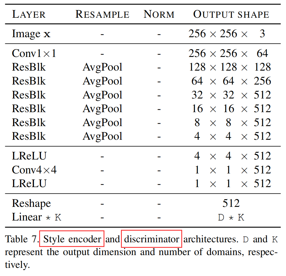
③、Style Encoder

其结构与鉴别器相同，区别在于结构图中最后一个Linear层，鉴别器是用一个Conv1x1实现，Style Encoder是用多个nn.Linear()代替。

输入为图像x及其所属的domain y，输出为domain y下的x的风格编码s

代码如下：

class StyleEncoder(nn.Module):
    def __init__(self, img_size=256, style_dim=64, num_domains=2, max_conv_dim=512):
        super().__init__()
        dim_in = 2**14 // img_size
        blocks = []
        blocks += [nn.Conv2d(3, dim_in, 3, 1, 1)]

        repeat_num = int(np.log2(img_size)) - 2
        for _ in range(repeat_num):
            dim_out = min(dim_in*2, max_conv_dim)
            blocks += [ResBlk(dim_in, dim_out, downsample=True)]
            dim_in = dim_out

        blocks += [nn.LeakyReLU(0.2)]
        blocks += [nn.Conv2d(dim_out, dim_out, 4, 1, 0)]
        blocks += [nn.LeakyReLU(0.2)]
        self.shared = nn.Sequential(*blocks)

        self.unshared = nn.ModuleList()
        for _ in range(num_domains):
            self.unshared += [nn.Linear(dim_out, style_dim)]

    def forward(self, x, y):
        h = self.shared(x)
        h = h.view(h.size(0), -1)
        out = []
        for layer in self.unshared:
            out += [layer(h)]
        out = torch.stack(out, dim=1)  # (batch, num_domains, style_dim)
        idx = torch.LongTensor(range(y.size(0))).to(y.device)
        s = out[idx, y]  # (batch, style_dim)
        return s

④、Mapping network

8层MLP：

输入为随机噪声z以及目标domain y，输出为对应的风格编码s

 代码如下：

class MappingNetwork(nn.Module):
    def __init__(self, latent_dim=16, style_dim=64, num_domains=2):
        super().__init__()
        layers = []
        layers += [nn.Linear(latent_dim, 512)]
        layers += [nn.ReLU()]
        for _ in range(3):
            layers += [nn.Linear(512, 512)]
            layers += [nn.ReLU()]
        self.shared = nn.Sequential(*layers)

        self.unshared = nn.ModuleList()
        for _ in range(num_domains):
            self.unshared += [nn.Sequential(nn.Linear(512, 512),
                                            nn.ReLU(),
                                            nn.Linear(512, 512),
                                            nn.ReLU(),
                                            nn.Linear(512, 512),
                                            nn.ReLU(),
                                            nn.Linear(512, style_dim))]

    def forward(self, z, y):
        h = self.shared(z)
        out = []
        for layer in self.unshared:
            out += [layer(h)]
        out = torch.stack(out, dim=1)  # (batch, num_domains, style_dim)
        idx = torch.LongTensor(range(y.size(0))).to(y.device)
        s = out[idx, y]  # (batch, style_dim)
        return s

3.loss设置

1、对抗loss

 

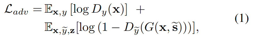
 对抗阶段：从高斯空间中采样得到一个高斯编码z，将该z和目标域的一个随机选取的图片y的风格关联起来。将z通过mapping net映射成一个风格向量，然后将该风格向量与x图片特征通过AdaIN变换融合，然后生成图片。通过判别器和生成器的对抗，一方面是是mapping net 输出更好的Y域风格向量y，另一方面是使得生成器能够学会利用风格向量s来生成Y域内更加真实的图片。

2、风格重建loss

风格重建：直觉就是，我将x的图片内容和风格y结合生成图片c，这时候我对c提取到的Y域风格特征应和之前的y尽量相同。这里使用了一个L1的loss。
这个loss的目的是为了使生成器在生成图片的时候保留风格y的特征。
本文与其他的风格提取网络的差别是本文的风格提取是多任务的。

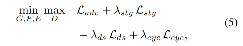
3、风格多样性loss

 风格差异：这是为了使得生成器搜素图像空间，发现更有意义的特征来生成多样性的图片，看公式就可以知道这是为了最大化生成图片两个域之间的风格特征的L1 loss。
不以分子分母的形式表示（相当于输入的风格特征的差距作为分母，生成图片的风格特征差距作为分子）是因为分母的轻微变换会导致该分数值很大，训练不稳定，因此才使用了文中的公式。
由于这种最大化是个很难确定的问题，所以这个loss的超参后面会降至0

4、重建loss

5、总的loss

4.训练过程

①、训练鉴别器

计算loss后，更新D的参数

②、训练生成器

计算loss后，更新E、M、G的参数

四.总结

star GAN的话只能根据每次变换一种属性风格，当没有属性标签时无法变换；而v2的话是变换域的风格，这是主要的区别。我觉得它就只是将前人的成果融合起来而已，主要的贡献是开源了一个动物数据。

starGAN v2 论文阅读_还是少年呀的博客-CSDN博客

2.有代码分析[CVPR2020] StarGAN v2：[CVPR2020] StarGAN v2_hellopipu的博客-CSDN博客_stargan v2

3.论文阅读】StarGAN v2：【论文阅读】StarGAN v2：Diverse Image Synthesis for Multiple Domains_huitailangyz的博客-CSDN博客

StarGAN第2版：多域多样性图像生成