a–c The molecular distributions defining the three complex molecular generative modeling task. 【a–c是在三项任务中分子分布图】 d–f examples of molecules from the training data in each of the generative modeling tasks.【d-f是三项任务中随机取的训练集样本】
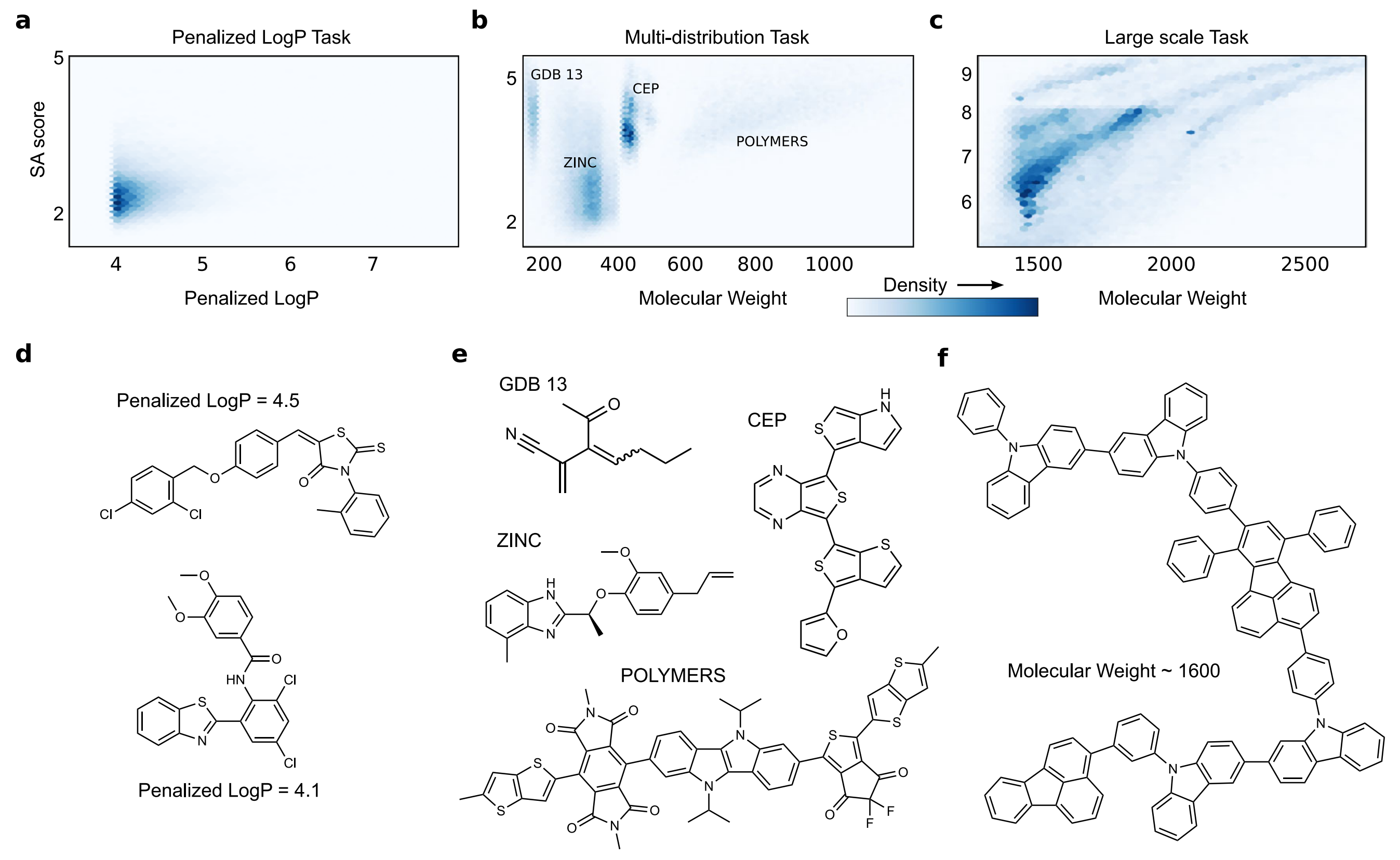
a The distribution of penalized LogP vs. SA score from the training data in the penalized logP task.【LogP 的分布规律,大多数位于4.0–4.5,10%超过6.0】
b The four modes of differently weighted molecules in the training data of the multi-distribution task.
c Large scale task’s molecular weight training distribution.
d The penalized LogP task,
e The multi-distribution task.
f The large-scale task.
1、惩罚 LogP 任务(Penalized LogP Task.)
the penalized LogP task是为了搜寻化学空间,学会了分子分布,就具有高的penalized LogP,该任务目标是学习具有高惩罚LogP分数的分子的分布。作者在ZINC数据库中筛选惩罚LogP值超过 4.0 的分子构建训练数据集(160K个),它们的LogP得分大多数是4.0–4.5。在分子训练数据集的尾部(大概占总数据集的10%),它们有更高的LogP 值(大于6.0)。
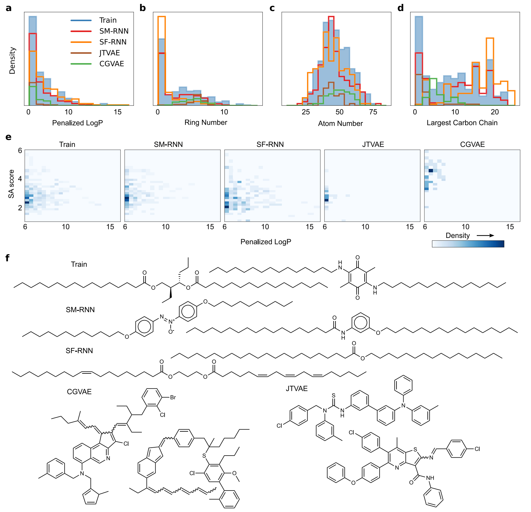
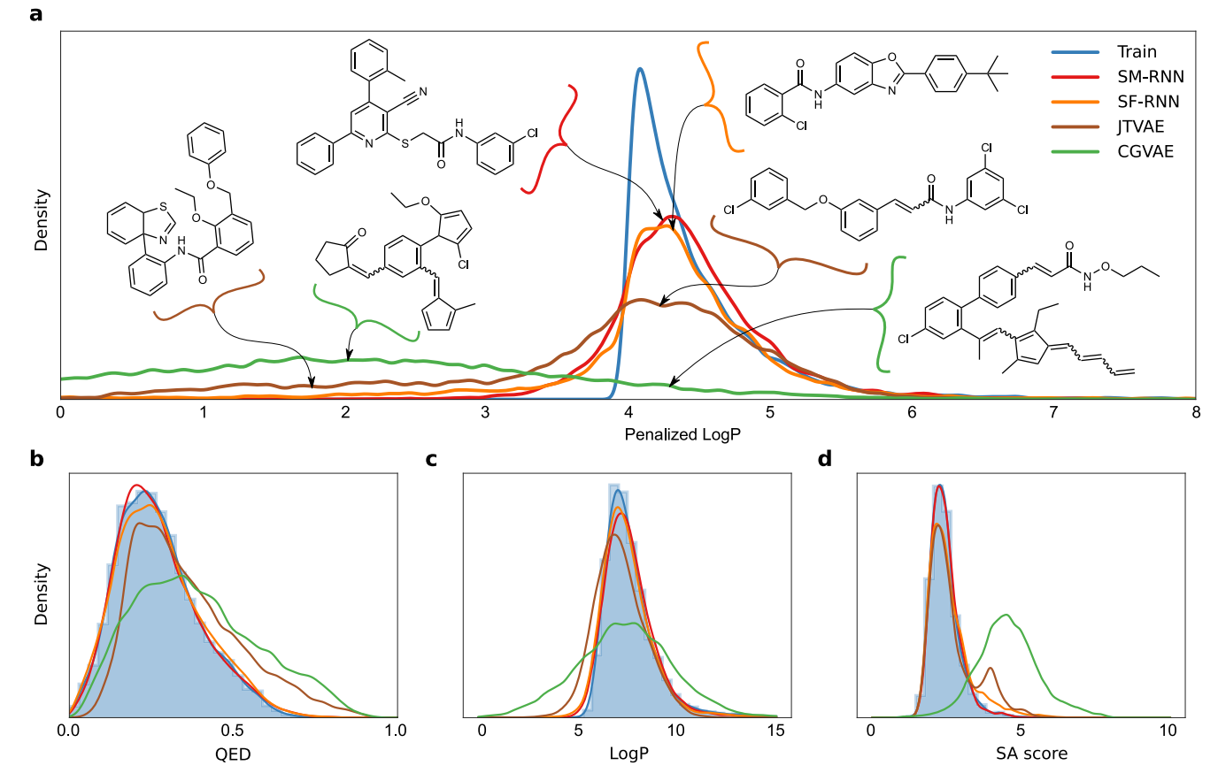
For the first task, we consider one of the most widely used benchmark assessments for searching chemical space, the penalized LogP task—finding molecules with high LogP penalized by synthesizability and unrealistic rings. We consider a generative modeling version of this task, where the goal is to learn distributions of molecules with high penalized LogP scores. Finding individual molecules with good scores (above 3.0) is a standard challenge but learning to directly generate from this part of chemical space, so that every molecule produced by the model has high penalized LogP, adds another degree of difficulty. For this we build a training dataset by screening the ZINC15 database for molecules with values of penalized LogP exceeding 4.0. Many machine learning approaches can only find a handful of molecules in this range, for example JTVAE found 22 total during all their attempts. After screening, the top scoring molecules in ZINC amounted to roughly 160K (K is thousand) molecules for the training data in this task. Thus, the training distribution is extremely spiked with most density falling around 4.0–4.5 penalized LogP as seen in Fig. 1a with most training molecules resembling the examplesshown in Fig. 1d. However, some of the training molecules, around 10% have even higher penalized LogP scores—adding a subtle tail to the distribution.
The results of training all models are shown in Figs. 2 and 3. The language models perform better than the graph models, with the SELFIES RNN producing a slightly closer match to the training distribution in Fig. 2a. The CGVAE and JTVAE learn to produce a large number of molecules with penalized LogP scores that are substantially worse than the lowest training scores. It is important to note, from the examples of these shown in Fig. 2a these lower scoring molecules are quite similar to the molecules from the main mode of the training distribution, this highlights the difficulty of learning this distribution. In Fig. 2b–d we see that JTVAE and CGVAE learn to produce more molecules with larger SA scores than the training data, as well, we see that all models learn the main mode of LogP in the training data but the RNNs produce closer distributions– similar results can be seen for QED. These results carryover for quantitative metrics and both RNNs achieve lower Wasserstein distance metrics than the CGVAE and JTVAE (Table 2) with the SMILES RNN coming closest to the TRAIN oracle.
图2 惩罚LogP任务结果I
a The plotted distribution of the penalized LogP scores of molecules from the training data (TRAIN) with the SM-RNN trained on SMILES, the SF-RNN trained on SELFIES and graph models: CGVAE and JTVAE. For the graph models we display molecules from the out of distribution mode at penalized LogP as well as molecules with penalized LogP score in the the main mode [4.0,4.5] from all models.【训练数据和测试的四个模型它们的LogP分布,分布越接近说明越拟合的越好】
b–d Distribution plots for all models and training data of molecular properties QED, LogP, and SA score.
表 2展示了(LogP, SA, QED, MW, BT, and NP这7种分子属性)Wasserstein距离 结果【其中TRAIN是一个oracle基础值,越接近它越好】,两个RNN生成的Wasserstein距离低于CGVAE和JTVAE,其中SM-RNN最接近最佳基准TRAIN。
We further investigate the highest penalized LogP region of the training data with values exceeding 6.0—the subtle tail of the training distribution. In the 2d distributions (Fig. 3e) it’s clear that both RNNs learn this subtle aspect of the training data while the graph models ignore it almost completely and only learnmolecules that are closer to the main mode. In particular, CGVAE learns molecules with larger SA score than the training data. Furthermore, the molecules with highest penalized LogP scores in the training data typically contain very long carbon chains and fewer rings (Fig. 3b, d)—the RNNs are capable of picking up on this. This is very apparent in the samples the model produce, a few are show in Fig. 3f, the RNNs produce mostly molecules with long carbon chains while the CGVAE and JTVAE generate molecules with many rings that have penalized LogP scores near 6.0. The language models learn a distribution that is close to the training distribution in the histograms of Fig. 3a–d. Overall, the language models could learn distributions of molecules with high penalized LogP scores, better than the graph models.
图3 惩罚LogP任务结果II
a–d Histograms of penalized LogP, Atoms #, Ring # and length of largest carbon chain (all per molecule) from molecules generated by all models or from the training data that have penalized LogP ≥ 6.0.【生成的分子和训练数据集的LogP, Atoms #, Ring # and length of largest carbon chain】
e 2d histograms of penalized LogP and SA score from molecules generated by the models or from training data that have penalized LogP ≥ 6.0.【生成的分子和训练数据集的LogP 和 SA得分】
f A few molecules generated by all models or from the training data that have penalized LogP ≥ 6.0.【四种模型生成的和训练数据集中的少量分子图】
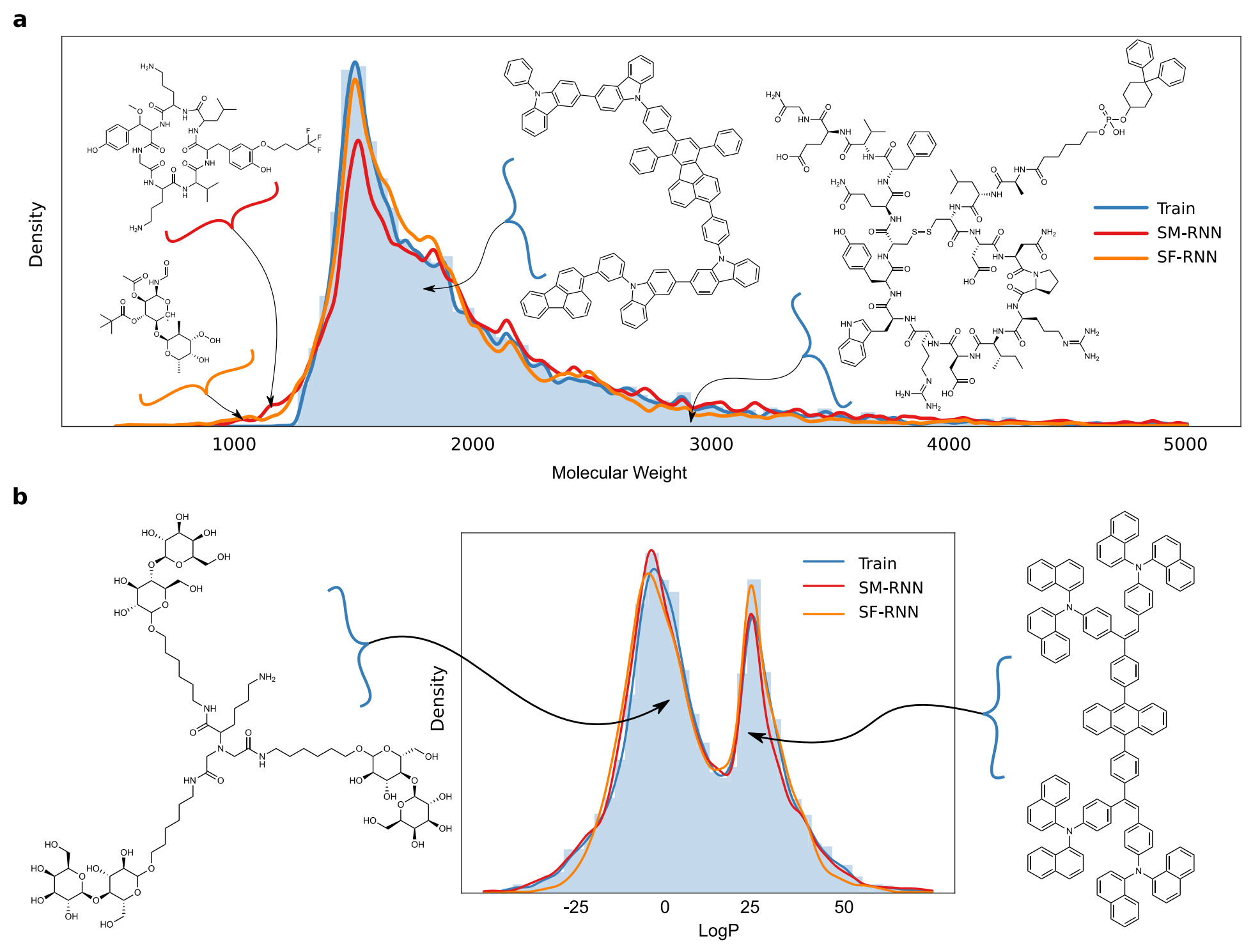
For the next task, we created a dataset by combining subsets of: (1) GDB13 molecules with molecular weight (MW) ≤ 185, (2) ZINC molecules with 185 ≤ MW ≤ 425, (3) Harvard clean energy project (CEP) molecules with 460 ≤ MW ≤ 600, and the (4) POLYMERS molecules with MW > 600. The training distribution has four modes– (Figs. 1b, e and 4a). CEP & GDB13 make up 1/3 and ZINC & POLYMERS take up 1/3 each of ∼200K training molecules.
In the multi-distribution task, both RNN models capture the data distribution quite well and learn every mode in the training distribution (Fig. 4a). On the other hand, JTVAE entirely misses the first mode from GDB13 then poorly learns ZINC and CEP. As well, CGVAE learns GDB13 but underestimates ZINC and entirely misses the mode from CEP. More evidence that the RNN models learn the training distribution more closely is apparent in Fig. 4e where CGVAE and JTVAE barely distinguish the main modes. Additionally, the RNN models generate molecules better resembling the training data (Supplementary Table 4). Despite this, all models– except CGVAE, capture the training distribution of QED, SA score and Bertz Complexity (Fig. 4b–d). Lastly, in Table 2 the RNN trained on SMILES has the lowest Wasserstein metrics followed by the SELFIES RNN then JTVAE and CGVAE.
图4 多分布任务结果
Fig4 Multi-distribution Task:
a The histogram and KDE of molecular weight of training molecules along with KDEs of molecular weight of molecules generated from all models. Three training molecules from each mode are shown.【在不同分子量(MW:Molecular Weight)的情况下,四个模型拟合train集的直方图】
b–d The histogram and KDE of QED, LogP and SA scores of training molecules along with KDES of molecules generated from all models.【4中模型捕获QED, LogP and Bertz Complexity分布的情况】
e 2d histograms of molecular weight and SA score of training molecules and molecules generated by all models.【在不同分子量(MW:Molecular Weight)的情况下,四个模型的SA得分,与train集更相似,说明RNN模型能更紧密地学习训练分布】
In addition, the training molecules seemed to be divided into two modes of molecules with lower and higher LogP values (Fig. 5b): with biomolecules defining the lower mode and molecules with more rings and longer carbons chains defining the higher LogP mode (more example molecules can be seen in supplementary Fig. 8). The RNN models were both able to learn the bi-modal nature of the training distribution.
图5 大规模任务结果I
Fig. 5 Large-scale Task I:
a The histogram and KDE of molecular weight of training molecules along with the KDEs of molecular weight of molecules generated from the RNNs. Two molecules generated by the RNN’s with lower molecular weight than the training molecules are shown on the left of the plot. In addition, two training molecules from the mode and tail of the distribution of molecular weight are displayed on the right.【大分子量的情况下,RNN可以很好地拟合训练分布】
b The histogram and KDE of LogP of training molecules along with the KDEs of LogP of molecules generated from the RNNs. On either side of the plot, for each mode in the LogP distribution, we display a molecule from the training data.【训练分子和从RNNs产生的分子的较低和较高LogP值的模式的直方图和KDE(核密度估计)。在图的任一侧,对于LogP分布中的每个模式,我们显示来自训练数据的一个分子。】
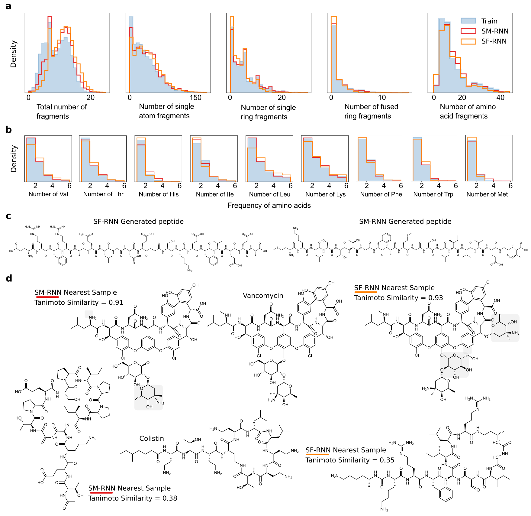
The training data has a variety of different molecules and substructures, in Fig. 6a the RNN models adequately learn the distribution of substructures arising in the training molecules. Specifically the distribution for the number of: fragments, single atom fragments as well as single, fused-ring and amino acid fragments in each molecule. As the training molecules get larger and occur less, both RNN models still learn to generate these molecules (Fig. 5a when molecular weigh >3000).
The dataset in this task contains a number of peptides and cyclic peptides that arise in PubChem, we visually analyze the samples from the RNNs to see if they are capable of preserving backbone chain structure and natural amino acids. We find that the RNNs often sample snippets of backbone chains which are usually disjoint—broken up with other atoms, bonds and structures. In addition, usually these chains have standard side chains from the main amino acid residues but other atypical side chains do arise. In Fig. 6c we show two examples of peptides that are generated by the SM-RNN and SF-RNN. While there are many examples where both models do not preserve backbone and fantasize weird side-chains, it is very likely, that if trained entirely on relevant peptides the model could be used for peptide design. Even further, since these language models are not restricted to generating amino acid sequences that could be used to design any biochemical structure that mimic the structure of peptics or even replicate their biological behavior. This makes them very applicable to design modified peptides, other peptide mimetics and complex natural products. The only requirement would be for a domain expert to construct a training dataset for specific targets. We conduct an additional study on how well the RNNs learned the biomolecular structures in the training data, in Fig. 6b we see both RNNs match the distribution of essential amino acid (found using a substructure search). Lastly, it is also likely that the RNNs could also be used to design cyclic peptides. To highlight the promise of language models for this task we display molecules generated by the RNNs with the largest Tanimoto similarity to colistin and vancomycin (Fig. 6d). The results in this task demonstrate that language models could be used to design more complex biomolecules.
图6 大规模任务结果II
Fig. 6 Large-scale Task II:
a Histograms of fragment #, single atom fragment #, single ring fragment #, fused-ring fragment #, amino acid fragment # (all per molecule) from molecules generated by the RNN models or from the training data.【RNN生成的子结构和训练集的分布状况,越匹配说明拟合的越好】
b Histograms of specific amino acid number in each molecule generated by the RNNs or from the training data.【由RNN生成的每个分子或训练集中特定氨基酸数量的直方图】
c A peptide generated by the SM-RNN—MKLSTTGFAMGSLIVVEGT (right) and one generated by the SFRNN—ERFRAQLGDEGSKEFVEEA (left).【由两种RNN生成的肽取例】
d Molecules generated by the SF-RNN and SM-RNN that are closest in Tanimoto similarity to colistin and vancomycin. The light gray shaded regions highlight differences from vancomycin.【展示了由SF-RNN和SM-RNN产生与粘菌素和万古霉素的Tanimoto相似性最接近的分子。浅灰色阴影区突出了与万古霉素的区别。这项任务的结果表明,语言模型可以用来设计更复杂的生物分子。】
We also evaluate models on standard metrics in the literature: validity, uniqueness and novelty. Using the same 10K molecules generated from each model for each task we compute the following statistics defined in ref. 17 and store them in Table 3: (1) validity: the ratio between the number of valid and generated molecules, (2) uniqueness: the ratio between the number of unique molecules (that are not duplicates) and valid molecules, (3) novelty: the ratio between unique molecules that are not in the training data and the total number of unique molecules. In the first two tasks (Table 3), JTVAE and CGVAE have better metrics with very high validity, uniqueness and novelty (all close to 1), here the SMILES and SELFIES RNN perform worse but the SELFIES RNN is close to their performance. The SMILES RNN has the worse metrics due to its poor grammar but is not substantially worse than the other models.


as well as molecules with penalized LogP score in the the main mode [4.0,4.5] from all models.【训练数据和测试的四个模型它们的LogP分布,分布越接近说明越拟合的越好】