更快更稳定的GAN训练高保真的小样本图像生成（ICLR 2021）

paper with code with supplement metrics：Towards Faster and Stabilized GAN Training for High-fidelity Few-shot Image Synthesis | OpenReview

official code：https://github.com/odegeasslbc/FastGAN-pytorch 

The video : https://www.youtube.com/watch?v=v8IRFcWGcWc

一、主要贡献：

The main contributions of the paper is：

1、a skip-layer excitation in the generator（SLE）：
We design the Skip-Layer channel-wise Excitation (SLE) module, which leverages low-scale activations to revise the channel responses on high-scale feature-maps. SLE allows a more robust gradient flow throughout the model weights for faster training. It also leads to an automated learning of a style/content disentanglement like StyleGAN2.

2、paired with autoencoding self-supervised learning in the discriminator：
We propose a self-supervised discriminator D trained as a feature-encoder with an extra decoder. We force D to learn a more descriptive feature-map covering more regions from an input image, thus yielding more comprehensive signals to train G. We test multiple self-supervision strategies for D, among which we show that auto-encoding works the best.
【这个鉴别器的设计很精妙，将D视作一个encoder，然后用一个小型decoder辅助训练】

Quoting the one-line summary "converge on single gpu with few hours' training, on 1024 resolution sub-hundred images".

二、提出本工作的起因和挑战

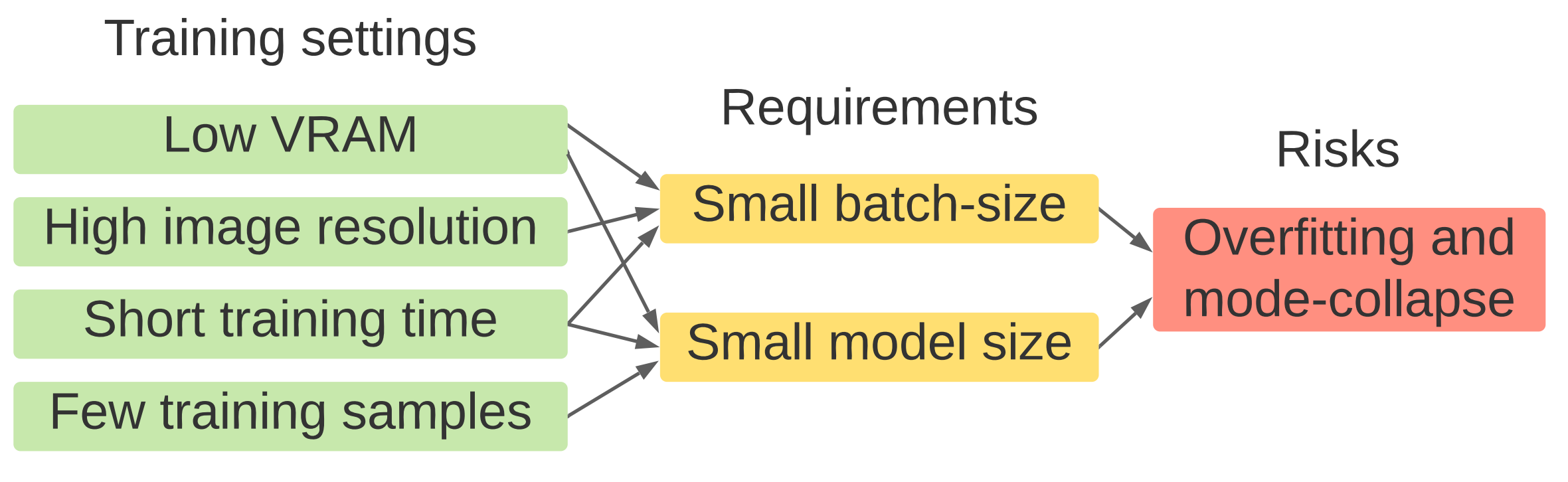
起因causes：低显存、高分辨率、短的训练时间、更少的训练样本

需求：小的batch-size、小的模型

挑战：过拟合、模型崩塌

三、模型结构

整体网络结构包含一个generator，一个discriminator。作者对generator做了精简，在每一个分辨率只包含了一个卷积层，在大于512分辨率的高层只使用了3通道。这些都使得模型训练速度很快，而且也不大（G和D总共155MB）。

1、Skip-Layer channel-wise Excitation（SLE）【ResBlock里的skip-layer的变种】

①▲、为什么做这样一个残差连接？

为了生成高分辨率的图像，G不可避免的要设计的更深，但是更深的卷积网络由于参数量的增加以及更慢的梯度更新速度会导致更多的训练时间。后来引入了残差连接，但是残差连接会导致更多的计算花费。作者由两个设计重新定义了残差连接：
1）、 原来的残差连接需要在不同的卷积激活层中使用 element-wise addition（逐元素相加），那么这个需要不同卷积激活层的维度相同才可以。与之前不同的是，这里作者使用的是 channel-wise multiplications（逐通道相乘）：消除了繁重的卷积计算（因为激活层具有的空间维度为1）
2）、在原来的工作中，残差连接只在一样的分辨率下使用，但在这里，作者使用跨分辨率的跳跃连接（例如：8-128,16-256）【可以看下TTSR，他也是跨层skip-connection】。由于是相乘，所以相同的维度这个条件就需要了，可以直接在不同的分辨率进行skip。
这样的话，SLE使网络既继承了ResBlock的 shortcut gradient flow的优势，与此同时还不需要这么大的计算负载。

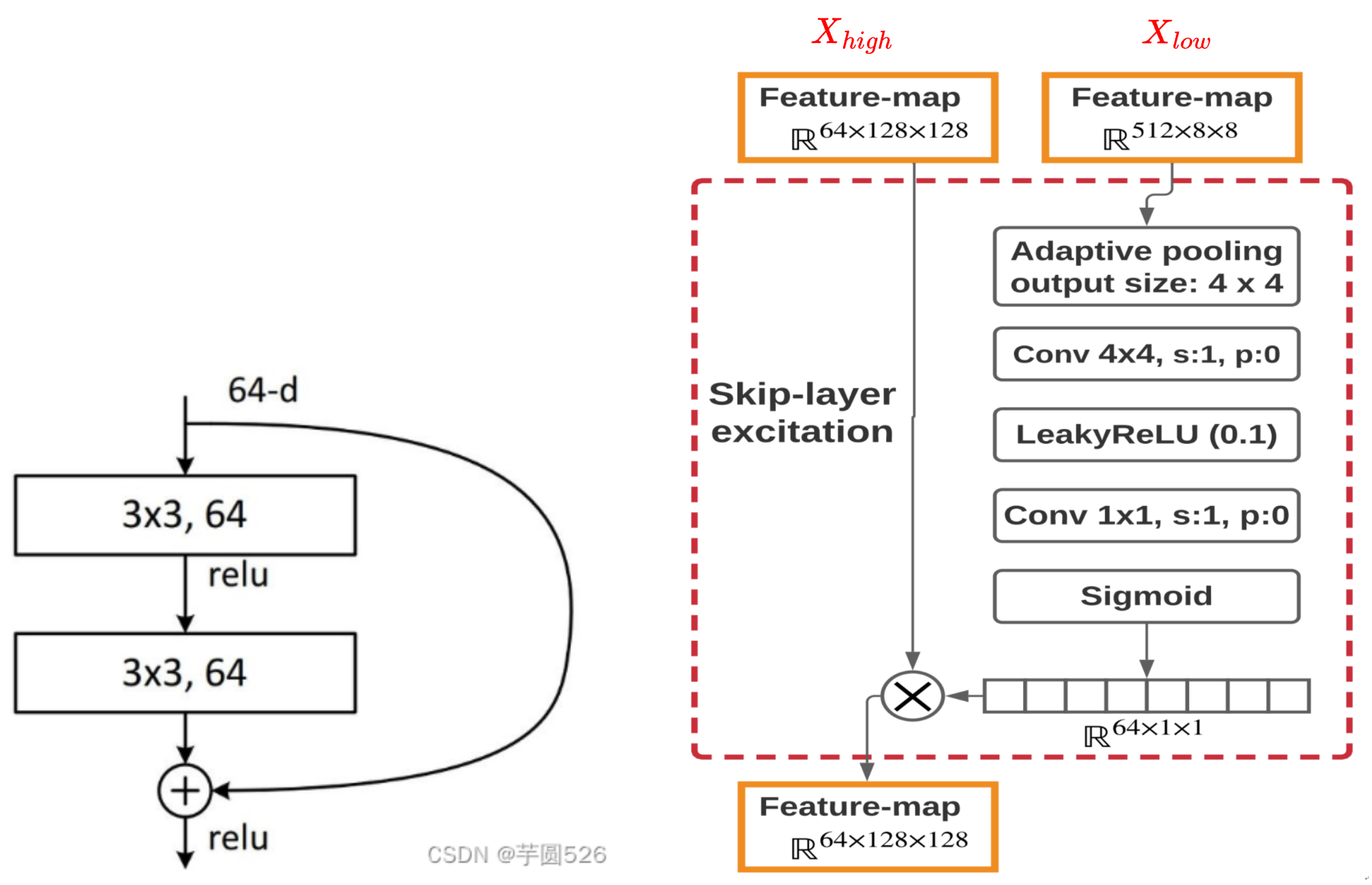
下图就是这个模块（SLE）的网络结构。下面详细介绍一下：

SLE公式为：

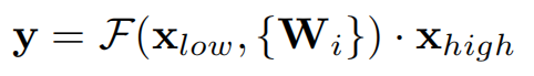
 这里 x 和 y 分别是SLE的输入和输出的特征图；
F 是对  的函数， 是要被学习的模型权重；
如上图所示， 和  分别代表8*8和128*128分辨率的特征图；

过程如下：

1. 首先F中的“adaptive average-pooling layer”先在空间维度将8*8“down-sample”为4*4；
2. 然后用一个4*4的Conv进一步“down-sample”为1*1；
3. 再使用LeakyReLU进行非线性操作；
4. 使用1*1的Conv将  的维度 和  保持一致；
5. 最后使用Sigmoid函数，F的输出沿通道的维度乘以 ，得到与  shape 相同的y（64x1x1 ☢ 64x128x128 = 64x128x128）

对比Skip-Layer Excitation（SLE）模块和ResBlock，有几个区别：

1. ResBlock最后是对两个特征图做的加法，而SLE做的是乘法。加法要求两个特征图分辨率相同，而乘法则没有这个要求，节约了大量计算。
2. SLE拥有分离style和content的性质，它的输入有两个大小不一样的特征图  和 ，如果把小一点的特征图  改为style图片，就可以实现风格迁移。（ 控制content， 控制style）

2、生成器G

1. 使用Progressive growing 和 SLE 块
2. 对 Conv2d 使用 Spectrally normalized 提升训练的稳定性

然后我们再看G的整体结构，稍微对模型做一下修改，它就可以生成任意大小（局限于2的次方）的图片。

Yellow boxes represent feature-maps (we show the spatial size and omit the channel number), blue box and blue arrows represent the same up-sampling structure, red box contains the SLE module as illustrated on the top.

3、基于自监督学习的Discriminator D

1. 使用Progressive growing 和 SLE 块
2. Treated as an encoder and trained with small decoders.
3. Regularized using an unsupervised reconstruction loss on its intermediate feature representations, which is only trained on real samples.

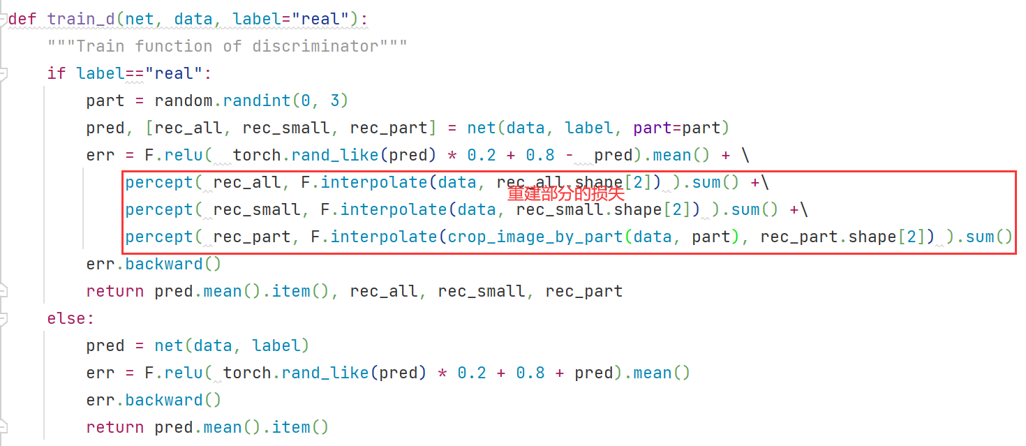
它的实现思路很简单：将D视作一个encoder，然后用一个小型decoder辅助训练。encoder从real image里提取特征，然后这些特征被输入到decoder里面要求根据特征重建图片。这样就可以迫使D学习到特征的准确性（全局的特征和局部的特征）。鉴别器D只在特征图 f1 16*16和特征图 f2 8*8上进行了Decoder，其中Decoder是由4个卷积层构成的从而重建为128*128的图像，这么做的目的是为了减少计算量。这里之所以叫self-supervisored learning 是因为auto-encoding这种方式是实现self-supervisored learning常用的方式，并且有利于提升模型的鲁棒性和生成能力。

Decoder的损失函数：只用了重建损失做训练。（公式里，G(f)是decoder从D提取的特征图再重建的图片，T(x)是对real sample做处理，使其可以计算损失），这里G和T的操作不仅仅局限于crop，更多的操作有待进行探索从而提升性能。

损失函数中计算重建损失在16*16的 f1 中使用的八分之一的图像求损失（为了减少计算量），在8*8的 f2 中不使用裁剪图像求损失；

1. We randomly crop f1 with1/8 of its height and width, then crop the real image on the same portion to get .
2. We resize the real image to get . The decoders produce from the cropped f1, and from f2.
3. Finally, D and the decoders are trained together to minimize the loss in eq. 2, by matching

思路和CycleGAN是有一些像的，只是本文里额外用了一个小decoder重建，而不是用G。（这样做的效果也许是减轻了运算压力？）
下面是整体D的结构。

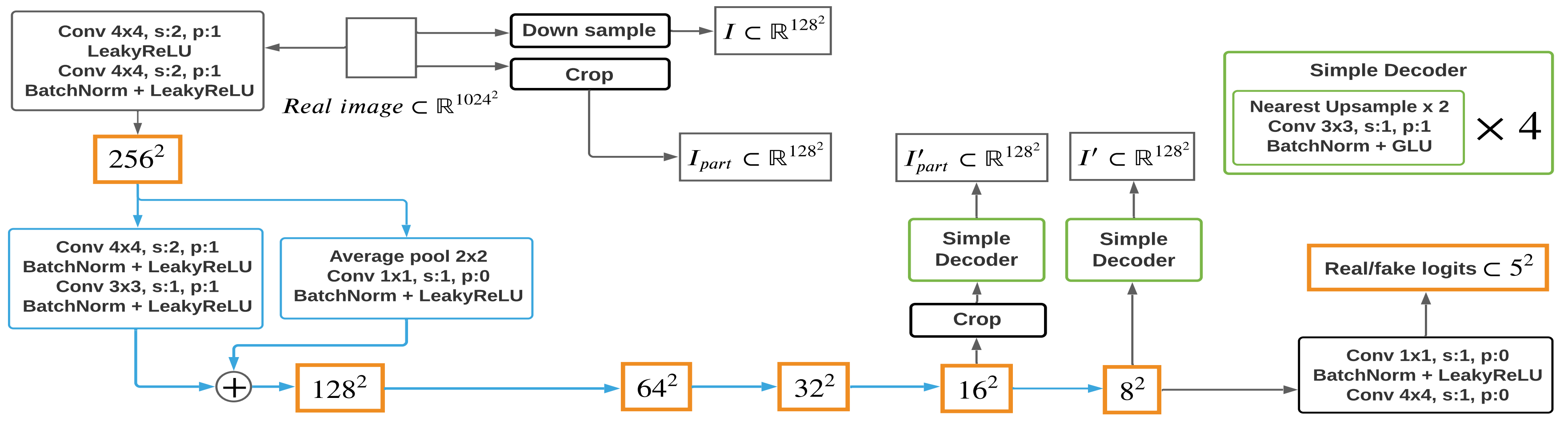
Blue box and arrows represent the same residual down-sampling structure, green boxes mean the same decoder structure

省去一些细节的部分，可以看到decoder是在16x16像素和8x8像素进行重建的，分别重建的是图片的局部和整体。（有一个奇怪的点是Loss一直没下降，所以会不会是D的问题？）

四、损失函数

G和D使用损失是： hinge version of the adversarial loss（GAN Hinge Loss）：GAN Hinge Loss Explained | Papers With Code

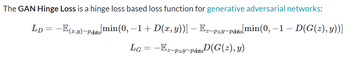
生成器和鉴别器的loss为：

4.1 鉴别器的损失

鉴别器的损失分为两部分组成：soft hinge loss（Rather hinge loss） prevent overfitting and mode collapse） + 重建损失

 1)soft hinge loss：（real + fake sample均进行训练）

 2)重建损失：(只在real sample上训练，不包含fake sample)

重建损失这里的损失函数使用的是perceptual similarity loss，而不是我当初想的“重建损失”(L1 loss)

4.2 生成器损失

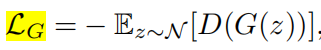
 In sum, we employ the hinge version of the adversarial loss to iteratively train our D and G. We find the different GAN losses make little performance difference, while hinge loss computes the fastest:

五、Experimence

1、MORE ANALYSIS AND APPLICATIONS

Testing mode collapse with back-tracking: From a well trained GAN, one can take a real image and invert it back to a vector in the latent space of G, thus editing the image’s content by altering the back-tracked vector. Despite the various back-tracking methods , a well generalized G is arguably as important for the good inversions. To this end, we show that our model, although trained on limited image samples, still gets a desirable performance on real image back-tracking.

 In Table 5, we split the images from each dataset with a training/testing ratio of 9:1, and train G on the training set. We compute a reconstruction error between all the images from the testing set and their inversions from G, after the same update of 1000 iterations on the latent vectors (to prevent the vectors from being far off the normal distribution). The baseline model’s performance is getting worse with more training iterations, which reflects mode-collapse on G. In contrast, our model gives better reconstructions with consistent performance over more training iterations. Fig. 6 presents the back-tracked examples (left-most and right-most samples in the middle panel) given the real images.

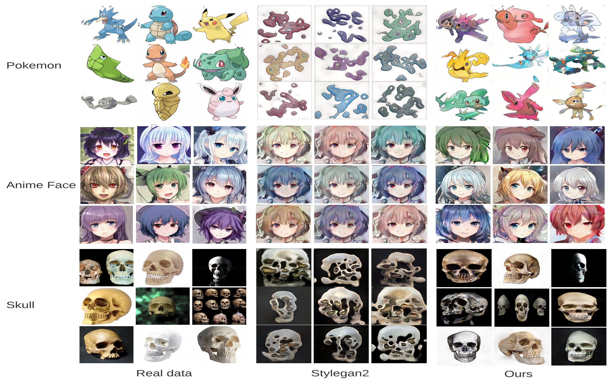
 Figure 5: Qualitative comparison between our model and StyleGAN2 on 1024*1024 resolution datasets. The left-most panel shows the training images, and the right two panels show the un-curated samples from StyleGAN2 and our model. Both models are trained from scratch for 10 hours with a batch-size of 8. The samples are generated from the checkpoint with the lowest FID.

【少样本图像生成】Towards Faster And Stabilized GAN training for high-fidelity few-shot image synthesis_芋圆526的博客-CSDN博客_少样本图像生成