
Aggregates in Pandas
In this lesson, you will learn about aggregates in Pandas. An aggregate statistic is a way of creating a single number that describes a group of numbers. Common aggregate statistics include mean, median, and standard deviation.
You will also learn how to rearrange a DataFrame into a pivot table, which is a great way to compare data across two dimensions.
# Before we analyze anything,we need to import pandas and load our data.

import pandas as pd

df = pd.read_csv('shoelfy_page_visits.csv')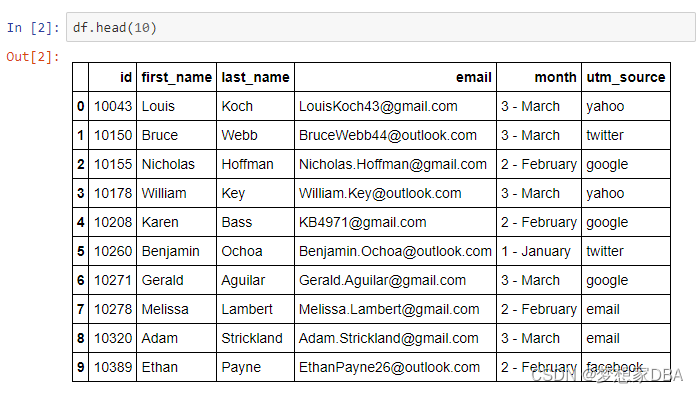
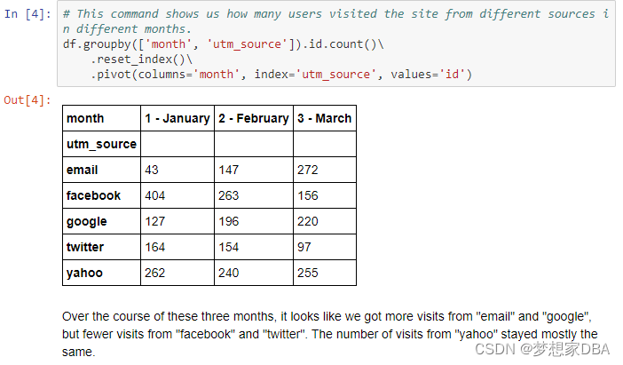
# This command shows us how many users visited the site from different sources in different months.
df.groupby(['month', 'utm_source']).id.count().reset_index()
Calculating Column Statistics
Aggregate functions summarize many data points (i.e., a column of a dataframe) into a smaller set of values.
Some examples of this type of calculation include:
- The DataFrame
customerscontains the names and ages of all of your customers. You want to find the median age:
print(customers.age)
>> [23, 25, 31, 35, 35, 46, 62]
print(customers.age.median())
>> 35- The DataFrame
shipmentscontains address information for all shipments that you’ve sent out in the past year. You want to know how many different states you have shipped to (and how many shipments went to the same state).
print(shipments.state)
>> ['CA', 'CA', 'CA', 'CA', 'NY', 'NY', 'NJ', 'NJ', 'NJ', 'NJ', 'NJ', 'NJ', 'NJ']
print(shipments.state.nunique())
>> 3
The DataFrame inventory contains a list of types of t-shirts that your company makes. You want a list of the colors that your shirts come in.
print(inventory.color)
>> ['blue', 'blue', 'blue', 'blue', 'blue', 'green', 'green', 'orange', 'orange', 'orange']
print(inventory.color.unique())
>> ['blue', 'green', 'orange']
The general syntax for these calculations is:
df.column_name.command()The following table summarizes some common commands:
| Command | Description |
|---|---|
mean | Average of all values in column |
std | Standard deviation |
median | Median |
max | Maximum value in column |
min | Minimum value in column |
count | Number of values in column |
nunique | Number of unique values in column |
unique | List of unique values in column |
1.Once more, we’ll revisit our orders from ShoeFly.com. Our new batch of orders is in the DataFrame orders. Examine the first 10 rows using the following code:
import codecademylib3
import pandas as pd

orders = pd.read_csv('orders.csv')
print(orders.head(10))
2.Our finance department wants to know the price of the most expensive pair of shoes purchased. Save your answer to the variable most_expensive.
import codecademylib3
import pandas as pd

orders = pd.read_csv('orders.csv')
print(orders.head(10))

most_expensive = orders.price.max()
3.Our fashion department wants to know how many different colors of shoes we are selling. Save your answer to the variable num_colors.
import codecademylib3
import pandas as pd

orders = pd.read_csv('orders.csv')
print(orders.head(10))

most_expensive = orders.price.max()

num_colors = orders.shoe_color.nunique()
Calculating Aggregate Functions I
When we have a bunch of data, we often want to calculate aggregate statistics (mean, standard deviation, median, percentiles, etc.) over certain subsets of the data.
Suppose we have a grade book with columns student, assignment_name, and grade. The first few lines look like this:
| student | assignment_name | grade |
|---|---|---|
| Amy | Assignment 1 | 75 |
| Amy | Assignment 2 | 35 |
| Bob | Assignment 1 | 99 |
| Bob | Assignment 2 | 35 |
| … | ||
We want to get an average grade for each student across all assignments. We could do some sort of loop, but Pandas gives us a much easier option: the method .groupby.
For this example, we’d use the following command:
grades = df.groupby('student').grade.mean()The output might look something like this:
| student | grade |
|---|---|
| Amy | 80 |
| Bob | 90 |
| Chris | 75 |
| … | |
In general, we use the following syntax to calculate aggregates:
df.groupby('column1').column2.measurement()where:
column1is the column that we want to group by ('student'in our example)column2is the column that we want to perform a measurement on (gradein our example)measurementis the measurement function we want to apply (meanin our example)
1.Let’s return to our orders data from ShoeFly.com.
In the previous exercise, our finance department wanted to know the most expensive shoe that we sold.
Now, they want to know the most expensive shoe for each shoe_type (i.e., the most expensive boot, the most expensive ballet flat, etc.).
Save your answer to the variable pricey_shoes.
2.Examine the object that you just created using:
print(pricey_shoes)3.What type of object is pricey_shoes?
Enter the following code to check:
print(type(pricey_shoes))
import codecademylib3
import pandas as pd

orders = pd.read_csv('orders.csv')
pricey_shoes = orders.groupby('shoe_type').price.max()
print(pricey_shoes)
print(type(pricey_shoes))
Calculating Aggregate Functions II
After using groupby, we often need to clean our resulting data.
As we saw in the previous exercise, the groupby function creates a new Series, not a DataFrame. For our ShoeFly.com example, the indices of the Series were different values of shoe_type, and the name property was price.
Usually, we’d prefer that those indices were actually a column. In order to get that, we can use reset_index(). This will transform our Series into a DataFrame and move the indices into their own column.
Generally, you’ll always see a groupby statement followed by reset_index:
df.groupby('column1').column2.measurement().reset_index()When we use groupby, we often want to rename the column we get as a result. For example, suppose we have a DataFrame teas containing data on types of tea:
| id | tea | category | caffeine | price |
|---|---|---|---|---|
| 0 | earl grey | black | 38 | 3 |
| 1 | english breakfast | black | 41 | 3 |
| 2 | irish breakfast | black | 37 | 2.5 |
| 3 | jasmine | green | 23 | 4.5 |
| 4 | matcha | green | 48 | 5 |
| 5 | camomile | herbal | 0 | 3 |
| … |
We want to find the number of each category of tea we sell. We can use:
teas_counts = teas.groupby('category').id.count().reset_index()This yields a DataFrame that looks like:
| category | id | |
|---|---|---|
| 0 | black | 3 |
| 1 | green | 4 |
| 2 | herbal | 8 |
| 3 | white | 2 |
| … | ||
The new column contains the counts of each category of tea sold. We have 3 black teas, 4 green teas, and so on. However, this column is called id because we used the id column of teas to calculate the counts. We actually want to call this column counts. Remember that we can rename columns:
teas_counts = teas_counts.rename(columns={"id": "counts"})Our DataFrame now looks like:
| category | counts | |
|---|---|---|
| 0 | black | 3 |
| 1 | green | 4 |
| 2 | herbal | 8 |
| 3 | white | 2 |
| … |
1.Modify your code from the previous exercise so that it ends with reset_index, which will change pricey_shoes into a DataFrame.
2.Examine the object that you’ve just created using the following code:
print(pricey_shoes)3.Now, what type of object is pricey_shoes?
Enter the following code to check:
print(type(pricey_shoes))import codecademylib3
import pandas as pd
orders = pd.read_csv('orders.csv')
pricey_shoes = orders.groupby('shoe_type').price.max().reset_index()
print(pricey_shoes)
print(type(pricey_shoes))Calculating Aggregate Functions III
Sometimes, the operation that you want to perform is more complicated than mean or count. In those cases, you can use the apply method and lambda functions, just like we did for individual column operations. Note that the input to our lambda function will always be a list of values.
A great example of this is calculating percentiles. Suppose we have a DataFrame of employee information called df that has the following columns:
id: the employee’s id numbername: the employee’s namewage: the employee’s hourly wagecategory: the type of work that the employee does
Our data might look something like this:
| id | name | wage | category |
|---|---|---|---|
| 10131 | Sarah Carney | 39 | product |
| 14189 | Heather Carey | 17 | design |
| 15004 | Gary Mercado | 33 | marketing |
| 11204 | Cora Copaz | 27 | design |
| … |
If we want to calculate the 75th percentile (i.e., the point at which 75% of employees have a lower wage and 25% have a higher wage) for each category, we can use the following combination of apply and a lambda function:
# np.percentile can calculate any percentile over an array of values
high_earners = df.groupby('category').wage
    .apply(lambda x: np.percentile(x, 75))
    .reset_index()
The output, high_earners might look like this:
| category | wage | |
|---|---|---|
| 0 | design | 23 |
| 1 | marketing | 35 |
| 2 | product | 48 |
| … |
1.Once more, we’ll return to the data from ShoeFly.com. Our Marketing team says that it’s important to have some affordably priced shoes available for every color of shoe that we sell.
Let’s calculate the 25th percentile for shoe price for each shoe_color to help Marketing decide if we have enough cheap shoes on sale. Save the data to the variable cheap_shoes.
Note: Be sure to use reset_index() at the end of your query so that cheap_shoes is a DataFrame.
2.Display cheap_shoes using print.
import codecademylib3
import numpy as np
import pandas as pd

orders = pd.read_csv('orders.csv')
cheap_shoes = orders.groupby('shoe_color').price.apply(lambda x: np.percentile(x,25)).reset_index()

print(cheap_shoes)
Calculating Aggregate Functions IV
Sometimes, we want to group by more than one column. We can easily do this by passing a list of column names into the groupby method.
Imagine that we run a chain of stores and have data about the number of sales at different locations on different days:
| Location | Date | Day of Week | Total Sales |
|---|---|---|---|
| West Village | February 1 | W | 400 |
| West Village | February 2 | Th | 450 |
| Chelsea | February 1 | W | 375 |
| Chelsea | February 2 | Th | 390 |
We suspect that sales are different at different locations on different days of the week. In order to test this hypothesis, we could calculate the average sales for each store on each day of the week across multiple months. The code would look like this:
df.groupby(['Location', 'Day of Week'])['Total Sales'].mean().reset_index()The results might look something like this:
| Location | Day of Week | Total Sales |
|---|---|---|
| Chelsea | M | 402.50 |
| Chelsea | Tu | 422.75 |
| Chelsea | W | 452.00 |
| … | ||
| West Village | M | 390 |
| West Village | Tu | 400 |
| … |
1.At ShoeFly.com, our Purchasing team thinks that certain shoe_type/shoe_color combinations are particularly popular this year (for example, blue ballet flats are all the rage in Paris).
Create a DataFrame with the total number of shoes of each shoe_type/shoe_color combination purchased. Save it to the variable shoe_counts.
You should be able to do this using groupby and count().
Note: When we’re using count(), it doesn’t really matter which column we perform the calculation on. You should use id in this example, but we would get the same answer if we used shoe_type or last_name.
Remember to use reset_index() at the end of your code!
2.Display shoe_counts using print.
import codecademylib3
import numpy as np
import pandas as pd

orders = pd.read_csv('orders.csv')

shoe_counts = orders.groupby(['shoe_type','shoe_color']).id.count().reset_index()

print(shoe_counts)
Pivot Tables
When we perform a groupby across multiple columns, we often want to change how our data is stored. For instance, recall the example where we are running a chain of stores and have data about the number of sales at different locations on different days:
| Location | Date | Day of Week | Total Sales |
|---|---|---|---|
| West Village | February 1 | W | 400 |
| West Village | February 2 | Th | 450 |
| Chelsea | February 1 | W | 375 |
| Chelsea | February 2 | Th | 390 |
We suspected that there might be different sales on different days of the week at different stores, so we performed a groupby across two different columns (Location and Day of Week). This gave us results that looked like this:
| Location | Day of Week | Total Sales |
|---|---|---|
| Chelsea | M | 300 |
| Chelsea | Tu | 310 |
| Chelsea | W | 320 |
| Chelsea | Th | 290 |
| … | ||
| West Village | Th | 400 |
| West Village | F | 390 |
| West Village | Sa | 250 |
| … | ||
In order to test our hypothesis, it would be more useful if the table was formatted like this:
| Location | M | Tu | W | Th | F | Sa | Su |
|---|---|---|---|---|---|---|---|
| Chelsea | 400 | 390 | 250 | 275 | 300 | 150 | 175 |
| West Village | 300 | 310 | 350 | 400 | 390 | 250 | 200 |
| … |
Reorganizing a table in this way is called pivoting. The new table is called a pivot table.
In Pandas, the command for pivot is:
df.pivot(columns='ColumnToPivot',
         index='ColumnToBeRows',
         values='ColumnToBeValues')
For our specific example, we would write the command like this:
# First use the groupby statement:
unpivoted = df.groupby(['Location', 'Day of Week'])['Total Sales'].mean().reset_index()
# Now pivot the table
pivoted = unpivoted.pivot(
    columns='Day of Week',
    index='Location',
    values='Total Sales')
Just like with groupby, the output of a pivot command is a new DataFrame, but the indexing tends to be “weird”, so we usually follow up with .reset_index().
1.In the previous example, you created a DataFrame with the total number of shoes of each shoe_type/shoe_color combination purchased for ShoeFly.com.
The purchasing manager complains that this DataFrame is confusing.
Make it easier for her to compare purchases of different shoe colors of the same shoe type by creating a pivot table. Save your results to the variable shoe_counts_pivot.
Your table should look like this:
| shoe_type | black | brown | navy | red | white |
|---|---|---|---|---|---|
| ballet flats | … | … | … | … | … |
| sandals | … | … | … | … | … |
| stilettos | … | … | … | … | … |
| wedges | … | … | … | … | … |
Remember to use reset_index() at the end of your code!
2.Display shoe_counts_pivot using print.
import codecademylib3
import numpy as np
import pandas as pd

orders = pd.read_csv('orders.csv')

shoe_counts = orders.groupby(['shoe_type', 'shoe_color']).id.count().reset_index()
shoe_counts_pivot = shoe_counts.pivot(index='shoe_type',columns='shoe_color',values='id').reset_index()

print(shoe_counts_pivot)
1.Let’s examine some more data from ShoeFly.com. This time, we’ll be looking at data about user visits to the website (the same dataset that you saw in the introduction to this lesson).
The data is a DataFrame called user_visits. Use print and head() to examine the first few rows of the DataFrame.
2.The column utm_source contains information about how users got to ShoeFly’s homepage. For instance, if utm_source = Facebook, then the user came to ShoeFly by clicking on an ad on Facebook.com.
Use a groupby statement to calculate how many visits came from each of the different sources. Save your answer to the variable click_source.
Remember to use reset_index()!
3.Paste the following code into script.py so that you can see the results of your previous groupby:
print(click_source)4.Our Marketing department thinks that the traffic to our site has been changing over the past few months. Use groupby to calculate the number of visits to our site from each utm_source for each month. Save your answer to the variable click_source_by_month.
5.The head of Marketing is complaining that this table is hard to read. Use pivot to create a pivot table where the rows are utm_source and the columns are month. Save your results to the variable click_source_by_month_pivot.
It should look something like this:
| utm_source | 1 - January | 2 - February | 3 - March |
|---|---|---|---|
| … | … | … | |
| … | … | … | |
| … | … | … | |
| … | … | … | |
| yahoo | … | … | … |
Checkpoint 6 Passed
6.View your pivot table by pasting the following code into script.py:
print(click_source_by_month_pivot)import codecademylib3
import pandas as pd
user_visits = pd.read_csv('page_visits.csv')
print(user_visits.head())
click_source = user_visits.groupby('utm_source').id.count().reset_index()
print(click_source)
click_source_by_month = user_visits.groupby(['utm_source','month']).id.count().reset_index()
click_source_by_month_pivot = click_source_by_month.pivot(columns='month',index='utm_source',values='id').reset_index()
print(click_source_by_month_pivot)A/B Testing for ShoeFly.com
Our favorite online shoe store, ShoeFly.com is performing an A/B Test. They have two different versions of an ad, which they have placed in emails, as well as in banner ads on Facebook, Twitter, and Google. They want to know how the two ads are performing on each of the different platforms on each day of the week. Help them analyze the data using aggregate measures.
If you get stuck during this project or would like to see an experienced developer work through it, click “Get Unstuck“ to see a project walkthrough video.
import codecademylib3
import pandas as pd

ad_clicks = pd.read_csv('ad_clicks.csv')
print(ad_clicks.head())
ad_clicks.groupby('utm_source').user_id.count().reset_index()

ad_clicks['is_click'] = ~ad_clicks.ad_click_timestamp.isnull()

clicks_by_source = ad_clicks.groupby(['utm_source','is_click']).user_id.count().reset_index()

clicks_pivot = clicks_by_source.pivot(columns='is_click',index='utm_source',values='user_id').reset_index()

clicks_pivot['percent_clicked']=clicks_pivot[True] / (clicks_pivot[True] + clicks_pivot[False])
clicks_pivot_by_experimental_group=clicks_Pivot.groupby(['experimental_group','is_click']).user_id.count().reset_index()

a_clicks = ad_clicks[ad_clicks.experimental_group=='A']
a_clicks.groupby(['is_click','day']).pivot(columns='is_click').id.count().reset_index()
相关文章
- pandas-数据分析
- 做一个Pandas专家,教你如何用它高效处理大量数据
- pandas 左右边界切割 用merge join和concat合并Pandas中的数据
- pandas.DataFrame.to_sql
- numpy, pandas, scikit-learn cheat sheet (速查表)
- Python pandas库|任凭弱水三千,我只取一瓢饮(2)
- Python pandas库|任凭弱水三千,我只取一瓢饮(1)
- Python之pandas:特征工程中数据类型(object/category/bool/int32/int64/float64)的简介、数据类型转换四大方法、案例应用之详细攻略
- Py之Pandas:Python的pandas库简介、安装、使用方法详细攻略
- Python之pandas:对dataframe数据的时间日期格式类型字段进行标准化变换(比如将日期类型字段格式2014/1/1转换为2014-1-1)之详细攻略
- 成功解决<pandas.core.groupby.generic.DataFrameGroupBy object at 0x0000024489925F60>
- 100天精通Python(数据分析篇)——第66天:Pandas透视表基础+实战案例(pivot_table函数)
- 100天精通Python(数据分析篇)——第59天:Pandas读写json文件(read_json、to_json参数说明+代码实战)
- 已解决import pandas as pd导包报错
- 已解决FutureWarning: The frame.append method is deprecated and will be removed from pandas in a future
- Pandas 多进程处理数据,速度的确快了很多
- 【阶段二】Python数据分析Pandas工具使用08篇:探索性数据分析:数据的描述:数据的分散趋势与数据的分布形态
- Pandas 通过追加方式合并多个csv
- Lesson3——Pandas Series结构
- pandas isin no is in