【Seq2Seq】压缩填充序列、掩蔽、推理和 BLEU

 🔎大家好，我是Sonhhxg_柒，希望你看完之后，能对你有所帮助，不足请指正！共同学习交流🔎

📝个人主页－Sonhhxg_柒的博客_CSDN博客 📃

🎁欢迎各位→点赞👍 + 收藏⭐️ + 留言📝​

📣系列专栏 - 机器学习【ML】 自然语言处理【NLP】  深度学习【DL】

​

 🖍foreword

✔说明⇢本人讲解主要包括Python、机器学习（ML）、深度学习（DL）、自然语言处理（NLP）等内容。

如果你对这个系列感兴趣的话，可以关注订阅哟👋

文章目录

简介

准备数据

构建模型

编码器

Attention

解码器

Seq2Seq

Training the Seq2Seq Model

推理

 BLEU

---

简介

在本笔记本中，我们将对上一个笔记本中的模型添加一些改进 - 填充序列和遮罩。打包的填充序列用于告诉我们的 RNN 跳过编码器中的填充令牌。掩码会显式强制模型忽略某些值，例如对填充元素的注意力。这两种技术都常用于 NLP。

我们还将研究如何使用我们的模型进行推理，通过给它一个句子，看看它翻译它是什么，看看它在翻译每个单词时究竟在哪里注意。

最后，我们将使用BLEU指标来衡量翻译质量。

准备数据

首先，我们将像以前一样导入所有模块，并添加用于查看注意力的matplotlib模块。

import torch
import torch.nn as nn
import torch.optim as optim
import torch.nn.functional as F

from torchtext.legacy.datasets import Multi30k
from torchtext.legacy.data import Field, BucketIterator

import matplotlib.pyplot as plt
import matplotlib.ticker as ticker

import spacy
import numpy as np

import random
import math
import time

接下来，我们将设置随机种子的可重复性。

SEED = 1234

random.seed(SEED)
np.random.seed(SEED)
torch.manual_seed(SEED)
torch.cuda.manual_seed(SEED)
torch.backends.cudnn.deterministic = True

和以前一样，我们将导入 spaCy 并定义德语和英语分词器。

spacy_de = spacy.load('de_core_news_sm')
spacy_en = spacy.load('en_core_web_sm')

def tokenize_de(text):
    """
    将字符串中的德语文本标记化为字符串列表
    """
    return [tok.text for tok in spacy_de.tokenizer(text)]

def tokenize_en(text):
    """
    将字符串中的英语文本标记化为字符串列表
    """
    return [tok.text for tok in spacy_en.tokenizer(text)]

当使用打包的填充序列时，我们需要告诉PyTorch实际（非填充）序列有多长。对我们来说幸运的是，TorchText的字段对象允许我们使用include_lengths参数，这将导致我们的批处理.src成为元组。元组的第一个元素与之前相同，一批数字化的源句子作为张量，第二个元素是批处理中每个源句子的非填充长度。

SRC = Field(tokenize = tokenize_de, 
            init_token = '<sos>', 
            eos_token = '<eos>', 
            lower = True, 
            include_lengths = True)

TRG = Field(tokenize = tokenize_en, 
            init_token = '<sos>', 
            eos_token = '<eos>', 
            lower = True)

然后，我们加载数据。

train_data, valid_data, test_data = Multi30k.splits(exts = ('.de', '.en'), 
                                                    fields = (SRC, TRG))

并建立词汇量。

SRC.build_vocab(train_data, min_freq = 2)
TRG.build_vocab(train_data, min_freq = 2)

接下来，我们处理迭代器。

关于打包填充序列的一个怪癖是，批处理中的所有元素都需要按其非填充长度降序排序，即批处理中的第一个句子需要最长。我们使用迭代器的两个参数来处理这个问题，sort_within_batch它告诉迭代器需要对批处理的内容进行排序，sort_key一个函数，它告诉迭代器如何对批处理中的元素进行排序。这里，我们按 src 句子的长度排序。

BATCH_SIZE = 128

device = torch.device('cuda' if torch.cuda.is_available() else 'cpu')

train_iterator, valid_iterator, test_iterator = BucketIterator.splits(
    (train_data, valid_data, test_data), 
     batch_size = BATCH_SIZE,
     sort_within_batch = True,
     sort_key = lambda x : len(x.src),
     device = device)

构建模型

编码器

接下来，我们定义编码器。

此处的更改都在正向方法中。它现在接受源句子的长度以及句子本身。

嵌入源句子（在迭代器中自动填充）后，我们可以在其上使用pack_padded_sequence句子的长度。请注意，包含序列长度的张量必须是最新版本的 PyTorch 的 CPU 张量，我们显式地使用 to（'cpu'） 来执行此操作。然后packed_embedded将是我们打包的填充序列。然后可以正常提供给我们的RNN，它将返回packed_outputs，一个包含序列中所有隐藏状态的填充张量，而隐藏张量只是我们序列中的最后一个隐藏状态。隐藏是一个标准张量，没有以任何方式打包，唯一的区别是，由于输入是一个打包序列，这个张量来自序列中的最后一个非填充元素。

然后，我们使用pad_packed_sequence解packed_outputs，该pad_packed_sequence返回每个输出和每个输出的长度，这是我们不需要的。

输出的第一个维度是填充序列长度，但是由于使用填充的填充序列，当填充标记是输入时，张量的值将全部为零。

class Encoder(nn.Module):
    def __init__(self, input_dim, emb_dim, enc_hid_dim, dec_hid_dim, dropout):
        super().__init__()
        
        self.embedding = nn.Embedding(input_dim, emb_dim)        
        self.rnn = nn.GRU(emb_dim, enc_hid_dim, bidirectional = True)       
        self.fc = nn.Linear(enc_hid_dim * 2, dec_hid_dim)        
        self.dropout = nn.Dropout(dropout)
        
    def forward(self, src, src_len):
        
        #src = [src len, batch size]
        #src_len = [batch size]
        
        embedded = self.dropout(self.embedding(src))        
        #embedded = [src len, batch size, emb dim]
                
        # 需要明确地将lengths放在cpu上！
        packed_embedded = nn.utils.rnn.pack_padded_sequence(embedded, src_len.to('cpu'))                
        packed_outputs, hidden = self.rnn(packed_embedded)
                                 
        # packed_outputs是包含所有隐藏状态的打包序列
        # hidden现在来自批处理中的最后一个非填充元素             
        outputs, _ = nn.utils.rnn.pad_packed_sequence(packed_outputs) 
            
        # 输出现在是非打包序列，获得所有隐藏状态
        # 当输入是填充标记时，全部为零
            
        #outputs = [src len, batch size, hid dim * num directions]
        #hidden = [n layers * num directions, batch size, hid dim]
        
        #hidden is stacked [forward_1, backward_1, forward_2, backward_2, ...]
        #输出始终来自最后一层
        
        #hidden [-2, :, : ] is the last of the forwards RNN 
        #hidden [-1, :, : ] is the last of the backwards RNN
        
        # 初始解码器隐藏是前进和后退的最终隐藏状态
        # 通过线性层馈送的编码器 RNN
        hidden = torch.tanh(self.fc(torch.cat((hidden[-2,:,:], hidden[-1,:,:]), dim = 1)))
        
        #outputs = [src len, batch size, enc hid dim * 2]
        #hidden = [batch size, dec hid dim]
        
        return outputs, hidden

Attention

注意模块是我们计算源句子上的注意力值的地方。

以前，我们允许此模块“注意”源句子中的填充标记。但是，使用遮罩，我们可以强制注意力仅放在非填充元素上。

正向方法现在采用掩码输入。这是一个  [batch size, source sentence length]张量，当源句子标记不是填充标记时为 1，当它是填充标记时为 0。例如，如果源句子是["hello", "how", "are", "you", "?", <pad>, <pad>]，则掩码将是 [1， 1， 1， 1， 1， 1， 0， 0]。

我们在计算注意力之后，但在它被softmax函数归一化之前应用掩码。它是使用masked_fill应用的。这将填充第一个参数（mask == 0）为 true 的每个元素处的张量，并使用第二个参数 （-1e10） 给出的值。换句话说，它将采用未规范化的注意力值，并将填充元素上的注意力值更改为 -1e10。由于这些数字与其他值相比是微小的，因此它们在通过softmax层时将变为零，从而确保不注意源句子中的填充标记。

class Attention(nn.Module):
    def __init__(self, enc_hid_dim, dec_hid_dim):
        super().__init__()
        
        self.attn = nn.Linear((enc_hid_dim * 2) + dec_hid_dim, dec_hid_dim)
        self.v = nn.Linear(dec_hid_dim, 1, bias = False)
        
    def forward(self, hidden, encoder_outputs, mask):
        
        #hidden = [batch size, dec hid dim]
        #encoder_outputs = [src len, batch size, enc hid dim * 2]
        
        batch_size = encoder_outputs.shape[1]
        src_len = encoder_outputs.shape[0]
        
        # 重复解码器隐藏状态src_len次
        hidden = hidden.unsqueeze(1).repeat(1, src_len, 1)
  
        encoder_outputs = encoder_outputs.permute(1, 0, 2)
        
        #hidden = [batch size, src len, dec hid dim]
        #encoder_outputs = [batch size, src len, enc hid dim * 2]
        
        energy = torch.tanh(self.attn(torch.cat((hidden, encoder_outputs), dim = 2))) 
        
        #energy = [batch size, src len, dec hid dim]

        attention = self.v(energy).squeeze(2)
        
        #attention = [batch size, src len]
        
        attention = attention.masked_fill(mask == 0, -1e10)
        
        return F.softmax(attention, dim = 1)

解码器

解码器只需要一些小的更改。它需要接受源句子上的掩码，并将其传递给注意力模块。当我们想在推理过程中查看注意力的值时，我们也返回注意力张量。

class Decoder(nn.Module):
    def __init__(self, output_dim, emb_dim, enc_hid_dim, dec_hid_dim, dropout, attention):
        super().__init__()

        self.output_dim = output_dim
        self.attention = attention
        
        self.embedding = nn.Embedding(output_dim, emb_dim)
        
        self.rnn = nn.GRU((enc_hid_dim * 2) + emb_dim, dec_hid_dim)
        
        self.fc_out = nn.Linear((enc_hid_dim * 2) + dec_hid_dim + emb_dim, output_dim)
        
        self.dropout = nn.Dropout(dropout)
        
    def forward(self, input, hidden, encoder_outputs, mask):
             
        #input = [batch size]
        #hidden = [batch size, dec hid dim]
        #encoder_outputs = [src len, batch size, enc hid dim * 2]
        #mask = [batch size, src len]
        
        input = input.unsqueeze(0)
        
        #input = [1, batch size]
        
        embedded = self.dropout(self.embedding(input))
        
        #embedded = [1, batch size, emb dim]
        
        a = self.attention(hidden, encoder_outputs, mask)
                
        #a = [batch size, src len]
        
        a = a.unsqueeze(1)
        
        #a = [batch size, 1, src len]
        
        encoder_outputs = encoder_outputs.permute(1, 0, 2)
        
        #encoder_outputs = [batch size, src len, enc hid dim * 2]
        
        weighted = torch.bmm(a, encoder_outputs)
        
        #weighted = [batch size, 1, enc hid dim * 2]
        
        weighted = weighted.permute(1, 0, 2)
        
        #weighted = [1, batch size, enc hid dim * 2]
        
        rnn_input = torch.cat((embedded, weighted), dim = 2)
        
        #rnn_input = [1, batch size, (enc hid dim * 2) + emb dim]
            
        output, hidden = self.rnn(rnn_input, hidden.unsqueeze(0))
        
        #output = [seq len, batch size, dec hid dim * n directions]
        #hidden = [n layers * n directions, batch size, dec hid dim]
        
        #seq len, n layers and n directions will always be 1 in this decoder, therefore:
        #output = [1, batch size, dec hid dim]
        #hidden = [1, batch size, dec hid dim]
        #this also means that output == hidden
        assert (output == hidden).all()
        
        embedded = embedded.squeeze(0)
        output = output.squeeze(0)
        weighted = weighted.squeeze(0)
        
        prediction = self.fc_out(torch.cat((output, weighted, embedded), dim = 1))
        
        #prediction = [batch size, output dim]
        
        return prediction, hidden.squeeze(0), a.squeeze(1)

Seq2Seq

总体 seq2seq 模型还需要对填充序列、屏蔽和推理进行一些更改。

我们需要告诉它 pad 令牌的索引是什么，并且还将源句子长度作为输入传递给 forward 方法。

我们使用 pad 令牌索引来创建掩码，方法是在源句子不等于 pad 标记的情况下创建一个 1 的掩码张量。这一切都在create_mask函数中完成。

序列长度根据需要传递到编码器以使用填充序列。

每个时间步长的注意力都存储在注意力中

class Seq2Seq(nn.Module):
    def __init__(self, encoder, decoder, src_pad_idx, device):
        super().__init__()
        
        self.encoder = encoder
        self.decoder = decoder
        self.src_pad_idx = src_pad_idx
        self.device = device
        
    def create_mask(self, src):
        mask = (src != self.src_pad_idx).permute(1, 0)
        return mask
        
    def forward(self, src, src_len, trg, teacher_forcing_ratio = 0.5):
        
        #src = [src len, batch size]
        #src_len = [batch size]
        #trg = [trg len, batch size]
        #teacher_forcing_ratio is probability to use teacher forcing
        #e.g. if teacher_forcing_ratio is 0.75 we use teacher forcing 75% of the time
                    
        batch_size = src.shape[1]
        trg_len = trg.shape[0]
        trg_vocab_size = self.decoder.output_dim
        
        #tensor to store decoder outputs
        outputs = torch.zeros(trg_len, batch_size, trg_vocab_size).to(self.device)
        
        #encoder_outputs is all hidden states of the input sequence, back and forwards
        #hidden is the final forward and backward hidden states, passed through a linear layer
        encoder_outputs, hidden = self.encoder(src, src_len)
                
        #first input to the decoder is the <sos> tokens
        input = trg[0,:]
        
        mask = self.create_mask(src)

        #mask = [batch size, src len]
                
        for t in range(1, trg_len):
            
            #insert input token embedding, previous hidden state, all encoder hidden states 
            #  and mask
            #receive output tensor (predictions) and new hidden state
            output, hidden, _ = self.decoder(input, hidden, encoder_outputs, mask)
            
            #place predictions in a tensor holding predictions for each token
            outputs[t] = output
            
            #decide if we are going to use teacher forcing or not
            teacher_force = random.random() < teacher_forcing_ratio
            
            #get the highest predicted token from our predictions
            top1 = output.argmax(1) 
            
            #if teacher forcing, use actual next token as next input
            #if not, use predicted token
            input = trg[t] if teacher_force else top1
            
        return outputs

Training the Seq2Seq Model

接下来，初始化模型并将其放置在 GPU 上。

INPUT_DIM = len(SRC.vocab)
OUTPUT_DIM = len(TRG.vocab)
ENC_EMB_DIM = 256
DEC_EMB_DIM = 256
ENC_HID_DIM = 512
DEC_HID_DIM = 512
ENC_DROPOUT = 0.5
DEC_DROPOUT = 0.5
SRC_PAD_IDX = SRC.vocab.stoi[SRC.pad_token]

attn = Attention(ENC_HID_DIM, DEC_HID_DIM)
enc = Encoder(INPUT_DIM, ENC_EMB_DIM, ENC_HID_DIM, DEC_HID_DIM, ENC_DROPOUT)
dec = Decoder(OUTPUT_DIM, DEC_EMB_DIM, ENC_HID_DIM, DEC_HID_DIM, DEC_DROPOUT, attn)

model = Seq2Seq(enc, dec, SRC_PAD_IDX, device).to(device)

然后，我们初始化模型参数。

def init_weights(m):
    for name, param in m.named_parameters():
        if 'weight' in name:
            nn.init.normal_(param.data, mean=0, std=0.01)
        else:
            nn.init.constant_(param.data, 0)
            
model.apply(init_weights)

Seq2Seq(
  (encoder): Encoder(
    (embedding): Embedding(7853, 256)
    (rnn): GRU(256, 512, bidirectional=True)
    (fc): Linear(in_features=1024, out_features=512, bias=True)
    (dropout): Dropout(p=0.5, inplace=False)
  )
  (decoder): Decoder(
    (attention): Attention(
      (attn): Linear(in_features=1536, out_features=512, bias=True)
      (v): Linear(in_features=512, out_features=1, bias=False)
    )
    (embedding): Embedding(5893, 256)
    (rnn): GRU(1280, 512)
    (fc_out): Linear(in_features=1792, out_features=5893, bias=True)
    (dropout): Dropout(p=0.5, inplace=False)
  )
)

我们将打印出模型中可训练参数的数量，请注意，如果没有这些改进，它具有与模型完全相同的参数量。

def count_parameters(model):
    return sum(p.numel() for p in model.parameters() if p.requires_grad)

print(f'The model has {count_parameters(model):,} trainable parameters')

The model has 20,518,405 trainable parameters

然后，我们定义优化程序和标准。

条件的ignore_index必须是目标语言的 pad 标记的索引，而不是源语言。

optimizer = optim.Adam(model.parameters())

TRG_PAD_IDX = TRG.vocab.stoi[TRG.pad_token]

criterion = nn.CrossEntropyLoss(ignore_index = TRG_PAD_IDX)

接下来，我们将定义训练和评估循环。

由于我们对源字段使用include_lengths = True，因此 batch.src 现在是一个元组，其中第一个元素是表示句子的数值化张量，第二个元素是批处理中每个句子的长度。

我们的模型还返回每个解码时间步长的源句子批次上的注意力向量。我们不会在训练/评估期间使用这些，但稍后会进行推理。

def train(model, iterator, optimizer, criterion, clip):
    
    model.train()
    
    epoch_loss = 0
    
    for i, batch in enumerate(iterator):
        
        src, src_len = batch.src
        trg = batch.trg
        
        optimizer.zero_grad()
        
        output = model(src, src_len, trg)
        
        #trg = [trg len, batch size]
        #output = [trg len, batch size, output dim]
        
        output_dim = output.shape[-1]
        
        output = output[1:].view(-1, output_dim)
        trg = trg[1:].view(-1)
        
        #trg = [(trg len - 1) * batch size]
        #output = [(trg len - 1) * batch size, output dim]
        
        loss = criterion(output, trg)
        
        loss.backward()
        
        torch.nn.utils.clip_grad_norm_(model.parameters(), clip)
        
        optimizer.step()
        
        epoch_loss += loss.item()
        
    return epoch_loss / len(iterator)

def evaluate(model, iterator, criterion):
    
    model.eval()
    
    epoch_loss = 0
    
    with torch.no_grad():
    
        for i, batch in enumerate(iterator):

            src, src_len = batch.src
            trg = batch.trg

            output = model(src, src_len, trg, 0) #turn off teacher forcing
            
            #trg = [trg len, batch size]
            #output = [trg len, batch size, output dim]

            output_dim = output.shape[-1]
            
            output = output[1:].view(-1, output_dim)
            trg = trg[1:].view(-1)

            #trg = [(trg len - 1) * batch size]
            #output = [(trg len - 1) * batch size, output dim]

            loss = criterion(output, trg)

            epoch_loss += loss.item()
        
    return epoch_loss / len(iterator)

然后，我们将定义一个有用的函数来计时 epoch 需要多长时间。

def epoch_time(start_time, end_time):
    elapsed_time = end_time - start_time
    elapsed_mins = int(elapsed_time / 60)
    elapsed_secs = int(elapsed_time - (elapsed_mins * 60))
    return elapsed_mins, elapsed_secs

倒数第二步是训练我们的模型。请注意，作为我们的模型，它几乎花费了一半的时间，而没有在此笔记本中添加的改进。

N_EPOCHS = 10
CLIP = 1

best_valid_loss = float('inf')

for epoch in range(N_EPOCHS):
    
    start_time = time.time()
    
    train_loss = train(model, train_iterator, optimizer, criterion, CLIP)
    valid_loss = evaluate(model, valid_iterator, criterion)
    
    end_time = time.time()
    
    epoch_mins, epoch_secs = epoch_time(start_time, end_time)
    
    if valid_loss < best_valid_loss:
        best_valid_loss = valid_loss
        torch.save(model.state_dict(), 'tut4-model.pt')
    
    print(f'Epoch: {epoch+1:02} | Time: {epoch_mins}m {epoch_secs}s')
    print(f'\tTrain Loss: {train_loss:.3f} | Train PPL: {math.exp(train_loss):7.3f}')
    print(f'\t Val. Loss: {valid_loss:.3f} |  Val. PPL: {math.exp(valid_loss):7.3f}')

Epoch: 01 | Time: 0m 34s
	Train Loss: 5.059 | Train PPL: 157.452
	 Val. Loss: 4.768 |  Val. PPL: 117.634
Epoch: 02 | Time: 0m 33s
	Train Loss: 4.090 | Train PPL:  59.736
	 Val. Loss: 4.080 |  Val. PPL:  59.142
Epoch: 03 | Time: 0m 33s
	Train Loss: 3.332 | Train PPL:  28.003
	 Val. Loss: 3.591 |  Val. PPL:  36.280
Epoch: 04 | Time: 0m 34s
	Train Loss: 2.855 | Train PPL:  17.381
	 Val. Loss: 3.358 |  Val. PPL:  28.739
Epoch: 05 | Time: 0m 36s
	Train Loss: 2.477 | Train PPL:  11.905
	 Val. Loss: 3.248 |  Val. PPL:  25.748
Epoch: 06 | Time: 0m 35s
	Train Loss: 2.190 | Train PPL:   8.937
	 Val. Loss: 3.238 |  Val. PPL:  25.484
Epoch: 07 | Time: 0m 34s
	Train Loss: 1.955 | Train PPL:   7.067
	 Val. Loss: 3.158 |  Val. PPL:  23.519
Epoch: 08 | Time: 0m 36s
	Train Loss: 1.761 | Train PPL:   5.816
	 Val. Loss: 3.237 |  Val. PPL:  25.461
Epoch: 09 | Time: 0m 34s
	Train Loss: 1.608 | Train PPL:   4.993
	 Val. Loss: 3.309 |  Val. PPL:  27.352
Epoch: 10 | Time: 0m 34s
	Train Loss: 1.500 | Train PPL:   4.483
	 Val. Loss: 3.316 |  Val. PPL:  27.558

最后，我们从最佳验证损失中加载参数，并在测试集上获得结果。

我们获得了改进的测试困惑，同时速度几乎是其两倍！

model.load_state_dict(torch.load('tut4-model.pt'))

test_loss = evaluate(model, test_iterator, criterion)

print(f'| Test Loss: {test_loss:.3f} | Test PPL: {math.exp(test_loss):7.3f} |')

| Test Loss: 3.143 | Test PPL:  23.179 |

推理

现在，我们可以使用训练的模型来生成翻译。

注意：与纸上显示的示例相比，这些翻译将很差，因为它们使用1000的隐藏尺寸并训练4天！它们被精心挑选，以展示在足够大的模型上应该是什么样子的注意力。

我们的translate_sentence将执行以下操作：

确保我们的模型处于评估模式，它应该始终用于推理

• 如果源句子尚未标记化，则对其进行标记化（是字符串）
• 对源句子进行数值化
• 将其转换为张量并添加批处理维度
• 获取源句子的长度并转换为张量
• 将源句子馈送到编码器中
• 为源句子创建掩码
• 创建一个列表来保存输出句子，用<sos>标记初始化
• 创建一个张量来保存注意力值
• 虽然我们没有达到最大长度

• 获取输入张量，该张量应为<sos>或最后预测的标记
• 将输入、所有编码器输出、隐藏状态和掩码馈送到解码器中
• 存储注意力值
• 获取预测的下一个令牌
• 将预测添加到当前输出句子预测
• 如果预测是令牌，则中断<eos>

• 将输出句子从索引转换为标记
• 返回输出句子（<sos>删除标记）和序列上的注意值

def translate_sentence(sentence, src_field, trg_field, model, device, max_len = 50):

    model.eval()
        
    if isinstance(sentence, str):
        nlp = spacy.load('de')
        tokens = [token.text.lower() for token in nlp(sentence)]
    else:
        tokens = [token.lower() for token in sentence]

    tokens = [src_field.init_token] + tokens + [src_field.eos_token]
        
    src_indexes = [src_field.vocab.stoi[token] for token in tokens]
    
    src_tensor = torch.LongTensor(src_indexes).unsqueeze(1).to(device)

    src_len = torch.LongTensor([len(src_indexes)])
    
    with torch.no_grad():
        encoder_outputs, hidden = model.encoder(src_tensor, src_len)

    mask = model.create_mask(src_tensor)
        
    trg_indexes = [trg_field.vocab.stoi[trg_field.init_token]]

    attentions = torch.zeros(max_len, 1, len(src_indexes)).to(device)
    
    for i in range(max_len):

        trg_tensor = torch.LongTensor([trg_indexes[-1]]).to(device)
                
        with torch.no_grad():
            output, hidden, attention = model.decoder(trg_tensor, hidden, encoder_outputs, mask)

        attentions[i] = attention
            
        pred_token = output.argmax(1).item()
        
        trg_indexes.append(pred_token)

        if pred_token == trg_field.vocab.stoi[trg_field.eos_token]:
            break
    
    trg_tokens = [trg_field.vocab.itos[i] for i in trg_indexes]
    
    return trg_tokens[1:], attentions[:len(trg_tokens)-1]

接下来，我们将创建一个函数，该函数在生成的每个目标令牌的源句子上显示模型的注意力。

def display_attention(sentence, translation, attention):
    
    fig = plt.figure(figsize=(10,10))
    ax = fig.add_subplot(111)
    
    attention = attention.squeeze(1).cpu().detach().numpy()
    
    cax = ax.matshow(attention, cmap='bone')
   
    ax.tick_params(labelsize=15)
    
    x_ticks = [''] + ['<sos>'] + [t.lower() for t in sentence] + ['<eos>']
    y_ticks = [''] + translation
     
    ax.set_xticklabels(x_ticks, rotation=45)
    ax.set_yticklabels(y_ticks)

    ax.xaxis.set_major_locator(ticker.MultipleLocator(1))
    ax.yaxis.set_major_locator(ticker.MultipleLocator(1))

    plt.show()
    plt.close()

现在，我们将从数据集中获取一些翻译，看看我们的模型做得有多好。请注意，我们将在这里挑选示例，以便我们查看一些有趣的东西，但可以随意更改example_idx值以查看不同的示例。

首先，我们将从数据集中获取源和目标。

example_idx = 12

src = vars(train_data.examples[example_idx])['src']
trg = vars(train_data.examples[example_idx])['trg']

print(f'src = {src}')
print(f'trg = {trg}')

src = ['ein', 'schwarzer', 'hund', 'und', 'ein', 'gefleckter', 'hund', 'kämpfen', '.']
trg = ['a', 'black', 'dog', 'and', 'a', 'spotted', 'dog', 'are', 'fighting']

然后，我们将使用我们的translate_sentence函数来获得我们预测的翻译和注意力。我们通过在 x 轴上显示源句子，在 y 轴上显示预测的平移来以图形方式显示这一点。两个单词之间的交点处的正方形越轻，模型在翻译该目标单词时对该源单词的关注就越多。

下面是模型尝试翻译的一个例子，它得到了正确的翻译，除了变化是fighting到只是fighting。

translation, attention = translate_sentence(src, SRC, TRG, model, device)

print(f'predicted trg = {translation}')

predicted trg = ['a', 'black', 'dog', 'and', 'a', 'spotted', 'dog', 'fighting', '.', '<eos>']

display_attention(src, translation, attention)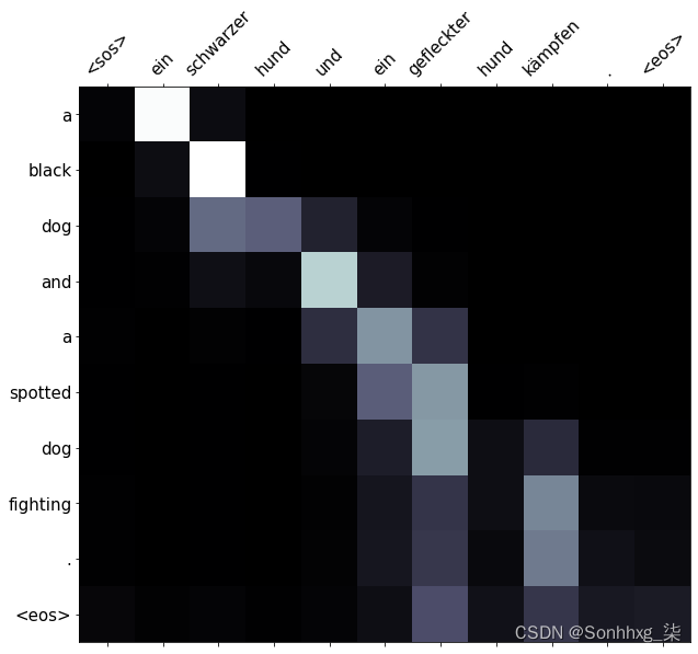

训练集中的翻译可以简单地由模型记忆。因此，我们查看验证和测试集的翻译也是公平的。

从验证集开始，让我们举个例子。

example_idx = 14

src = vars(valid_data.examples[example_idx])['src']
trg = vars(valid_data.examples[example_idx])['trg']

print(f'src = {src}')
print(f'trg = {trg}')

src = ['eine', 'frau', 'spielt', 'ein', 'lied', 'auf', 'ihrer', 'geige', '.']
trg = ['a', 'female', 'playing', 'a', 'song', 'on', 'her', 'violin', '.']

然后，让我们生成翻译并查看注意力。

在这里，我们可以看到翻译是一样的，除了交换女性和女人。

translation, attention = translate_sentence(src, SRC, TRG, model, device)

print(f'predicted trg = {translation}')

display_attention(src, translation, attention)

predicted trg = ['a', 'woman', 'playing', 'a', 'song', 'on', 'her', 'violin', '.', '<eos>']

 最后，让我们从测试集中得到一个示例。

example_idx = 18

src = vars(test_data.examples[example_idx])['src']
trg = vars(test_data.examples[example_idx])['trg']

print(f'src = {src}')
print(f'trg = {trg}')

src = ['die', 'person', 'im', 'gestreiften', 'shirt', 'klettert', 'auf', 'einen', 'berg', '.']
trg = ['the', 'person', 'in', 'the', 'striped', 'shirt', 'is', 'mountain', 'climbing', '.']

同样，它产生的翻译与目标略有不同，是源句子的更直白的版本。它把登山换成了爬山。

translation, attention = translate_sentence(src, SRC, TRG, model, device)

print(f'predicted trg = {translation}')

display_attention(src, translation, attention)

predicted trg = ['the', 'person', 'in', 'the', 'striped', 'shirt', 'is', 'climbing', 'a', 'mountain', '.', '<eos>']

 BLEU

以前，我们只关心模型的loss/perplexity。但是，有一些指标是专门为衡量翻译质量而设计的 - 最受欢迎的是BLEU。在不涉及太多细节的情况下，BLEU根据n-gram来查看预测和实际目标序列中的重叠。对于每个序列，它将为我们提供一个介于0和1之间的数字，其中1表示存在完美的重叠，即完美的翻译，尽管通常显示在0到100之间。BLEU是为每个源序列的多个候选翻译设计的，但是在此数据集中，每个源只有一个候选翻译。

我们定义了一个calculate_bleu函数，用于计算提供的TorchText数据集的BLEU分数。此函数为每个源句子创建实际和预测翻译的语料库，然后计算BLEU分数。

from torchtext.data.metrics import bleu_score

def calculate_bleu(data, src_field, trg_field, model, device, max_len = 50):
    
    trgs = []
    pred_trgs = []
    
    for datum in data:
        
        src = vars(datum)['src']
        trg = vars(datum)['trg']
        
        pred_trg, _ = translate_sentence(src, src_field, trg_field, model, device, max_len)
        
        #cut off <eos> token
        pred_trg = pred_trg[:-1]
        
        pred_trgs.append(pred_trg)
        trgs.append([trg])
        
    return bleu_score(pred_trgs, trgs)

我们得到大约28 BLEU。如果我们将其与注意力模型试图复制的论文进行比较，它们BLEU得分为26.75。这与我们的分数相似，但是他们使用的是完全不同的数据集，并且它们的模型大小要大得多 - 1000个隐藏维度，需要4天的训练时间！- 所以我们也不能真正与之相比。

这个数字并不是真正可以解释的，我们真的不能说太多。BLEU分数最有用的部分是，它可用于比较同一数据集上的不同模型，其中BLEU得分较高的模型“better”。

bleu_score = calculate_bleu(test_data, SRC, TRG, model, device)

print(f'BLEU score = {bleu_score*100:.2f}')

BLEU score = 28.11

在下一个教程中，我们将不再使用递归神经网络，并开始研究构建序列到序列模型的其他方法。具体来说，在下一教程中，我们将使用卷积神经网络。