实现主成分分析 （PCA） 和独立成分分析 （ICA） （Matlab代码实现）

 👨‍🎓个人主页：研学社的博客 

💥💥💞💞欢迎来到本博客❤️❤️💥💥

🏆博主优势：🌞🌞🌞博客内容尽量做到思维缜密，逻辑清晰，为了方便读者。

⛳️座右铭：行百里者，半于九十。

📋📋📋本文目录如下：🎁🎁🎁

目录

💥1 概述

📚2 运行结果

2.1 ICA

 2.2 PCA

🌈3 Matlab代码实现

🎉4 参考文献

---

💥1 概述

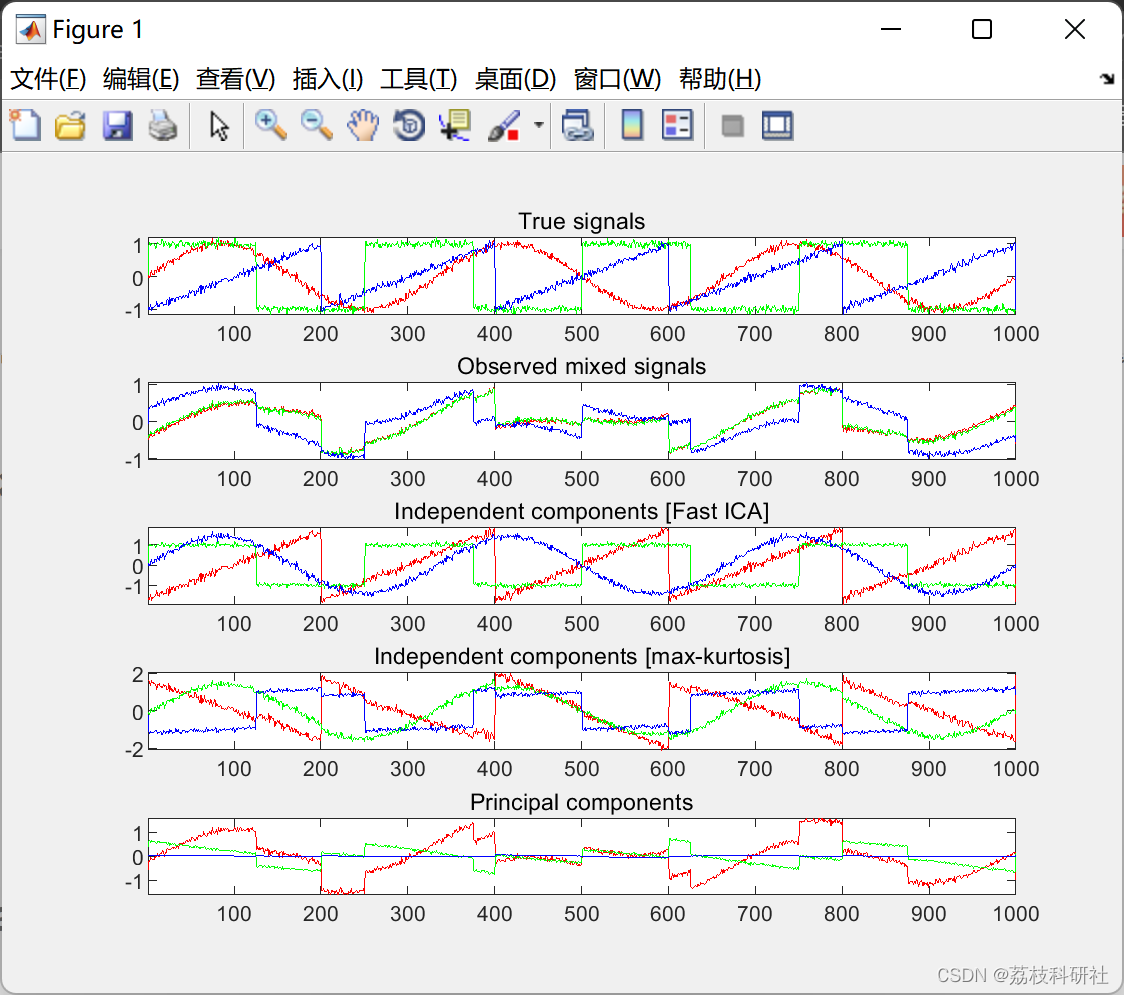
在PCA中，多维数据被投影到对应于其几个最大奇异值的奇异向量上。此类操作有效地将输入单分解为数据中方差最大的方向上的正交分量。因此，PCA通常用于降维应用，其中执行PCA会产生数据的低维表示，可以反转以紧密重建原始数据。
在 ICA 中，多维数据被分解为在适当意义上最大程度独立的组件（在此包中为峰度和负熵）。ICA与PCA的不同之处在于，低维信号不一定对应于最大方差的方向;相反，ICA组成部分具有最大的统计独立性。在实践中，ICA通常可以在多维数据中发现不相交的潜在趋势。

📚2 运行结果

2.1 ICA

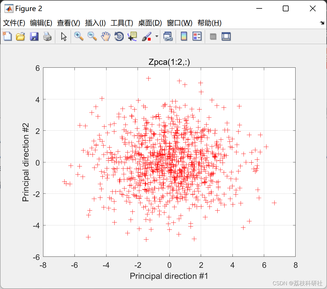
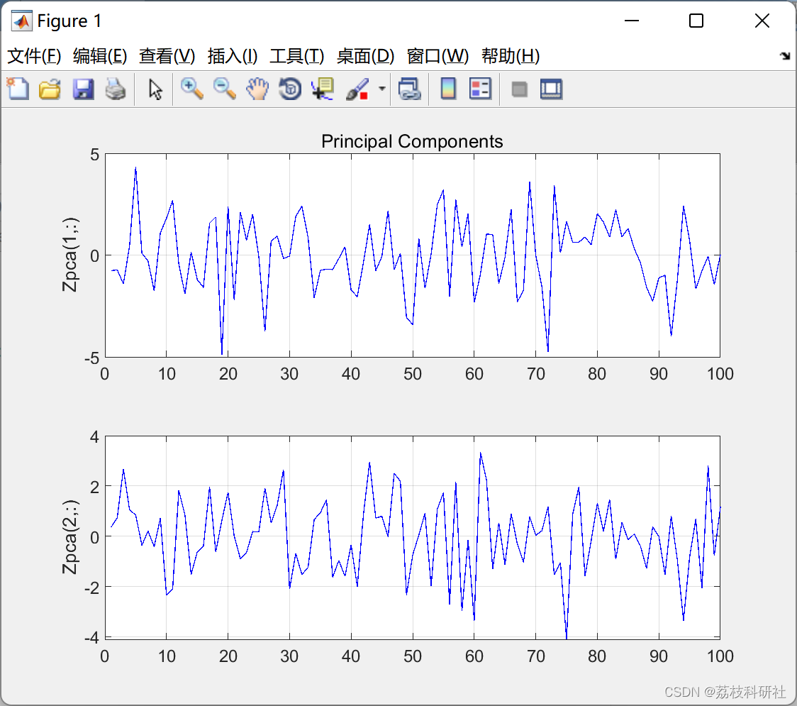
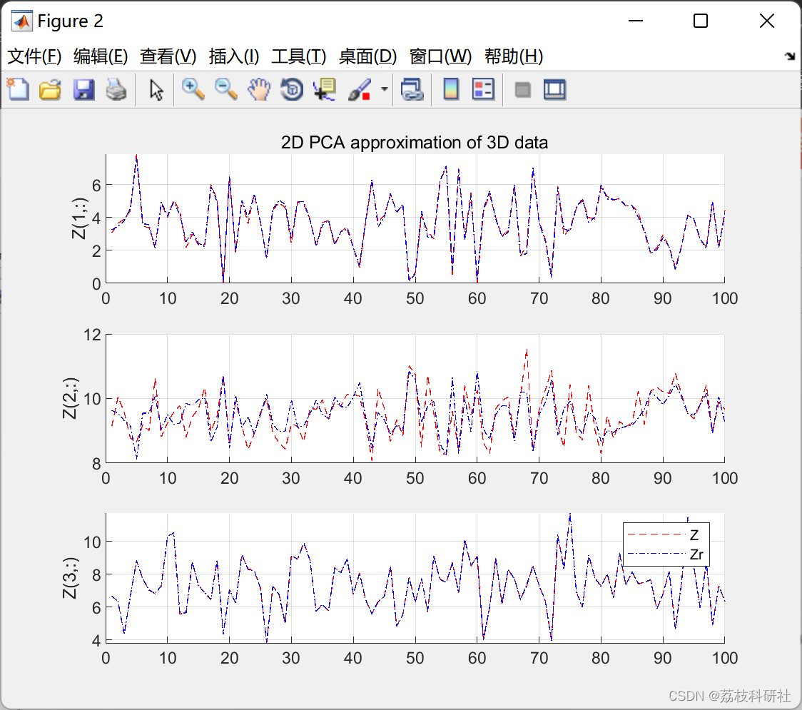
 2.2 PCA

部分代码：

% Knobs
n = 100;    % Number of samples
d = 3;      % Sample dimension
r = 2;      % Number of principal components

% Generate Gaussian data
MU = 10 * rand(d,1);
sigma = (2 * randi([0 1],d) - 1) .* rand(d);
SIGMA = 3 * (sigma * sigma');
Z = mvg(MU,SIGMA,n);

% Perform PCA
[Zpca, U, mu] = PCA(Z,r);
Zr = U * Zpca + repmat(mu,1,n);

% Plot principal components
figure;
for i = 1:r
    subplot(r,1,i);
    plot(Zpca(i,:),'b');
    grid on;
    ylabel(sprintf('Zpca(%i,:)',i));
end
subplot(r,1,1);
title('Principal Components');

% Plot r-dimensional approximations
figure;
for i = 1:d
    subplot(d,1,i);
    hold on;
    p1 = plot(Z(i,:),'--r');
    p2 = plot(Zr(i,:),'-.b');
    grid on;
    ylabel(sprintf('Z(%i,:)',i));
end
subplot(d,1,1);
title(sprintf('%iD PCA approximation of %iD data',r,d));
legend([p1 p2],'Z','Zr');
 

% Knobs
n = 100;    % Number of samples
d = 3;      % Sample dimension
r = 2;      % Number of principal components

% Generate Gaussian data
MU = 10 * rand(d,1);
sigma = (2 * randi([0 1],d) - 1) .* rand(d);
SIGMA = 3 * (sigma * sigma');
Z = mvg(MU,SIGMA,n);

% Perform PCA
[Zpca, U, mu] = PCA(Z,r);
Zr = U * Zpca + repmat(mu,1,n);

% Plot principal components
figure;
for i = 1:r
    subplot(r,1,i);
    plot(Zpca(i,:),'b');
    grid on;
    ylabel(sprintf('Zpca(%i,:)',i));
end
subplot(r,1,1);
title('Principal Components');

% Plot r-dimensional approximations
figure;
for i = 1:d
    subplot(d,1,i);
    hold on;
    p1 = plot(Z(i,:),'--r');
    p2 = plot(Zr(i,:),'-.b');
    grid on;
    ylabel(sprintf('Z(%i,:)',i));
end
subplot(d,1,1);
title(sprintf('%iD PCA approximation of %iD data',r,d));
legend([p1 p2],'Z','Zr');

🌈3 Matlab代码实现

🎉4 参考文献

部分理论来源于网络，如有侵权请联系删除。

[1]Brian Moore (2022). PCA and ICA Package