二氧化碳捕获和电化学转化（Python代码实现）

 👨‍🎓个人主页：研学社的博客 

💥💥💞💞欢迎来到本博客❤️❤️💥💥

🏆博主优势：🌞🌞🌞博客内容尽量做到思维缜密，逻辑清晰，为了方便读者。

⛳️座右铭：行百里者，半于九十。

📋📋📋本文目录如下：🎁🎁🎁

目录

💥1 概述

📚2 运行结果

 2.2 算例2

 2.3 算例3

 2.4 算例4

🎉3 参考文献

🌈4 Matlab代码实现

---

💥1 概述

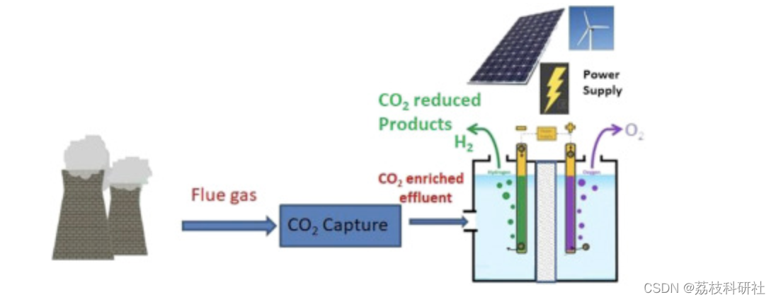
二氧化碳（二氧化碳需要大幅减少向大气中的排放，以遏制气候变化的各种不良影响。一种方法是从化石燃料发电厂转向太阳能、风能和水等可再生能源，这还有一个额外的好处，那就是我们减少了对全球化石燃料供应减少的依赖。然而，由于其间歇性，可再生能源可以提供的能源比例将限制在30%，除非有大规模储能的方法可用。或者，二氧化碳可以从发电厂等点源捕获，然后转化为具有经济价值的化学品[1，2，3]。潜在的产物包括甲酸[4••，5]，甲醇，CO[4••，6，7•，8，9，10，11，12，13••]和乙烯[4••，14•]，它们可以使用均相催化[15，16]，多相催化[17••，18]，光催化[19]，光还原[19]或电化学还原等工艺形成 - 这是本综述的主题。除了减少温室气体排放外，一氧化碳2转化过程将减少我们对化学合成化石燃料的依赖。然而，在这一点上，尚不清楚这些策略中哪些在技术上可行，并且具有经济和实践意义[1]。电化学二氧化碳减少的好处是，它可能是一种利用间歇性可再生能源的多余能量代替大规模储能的方法。

📚2 运行结果

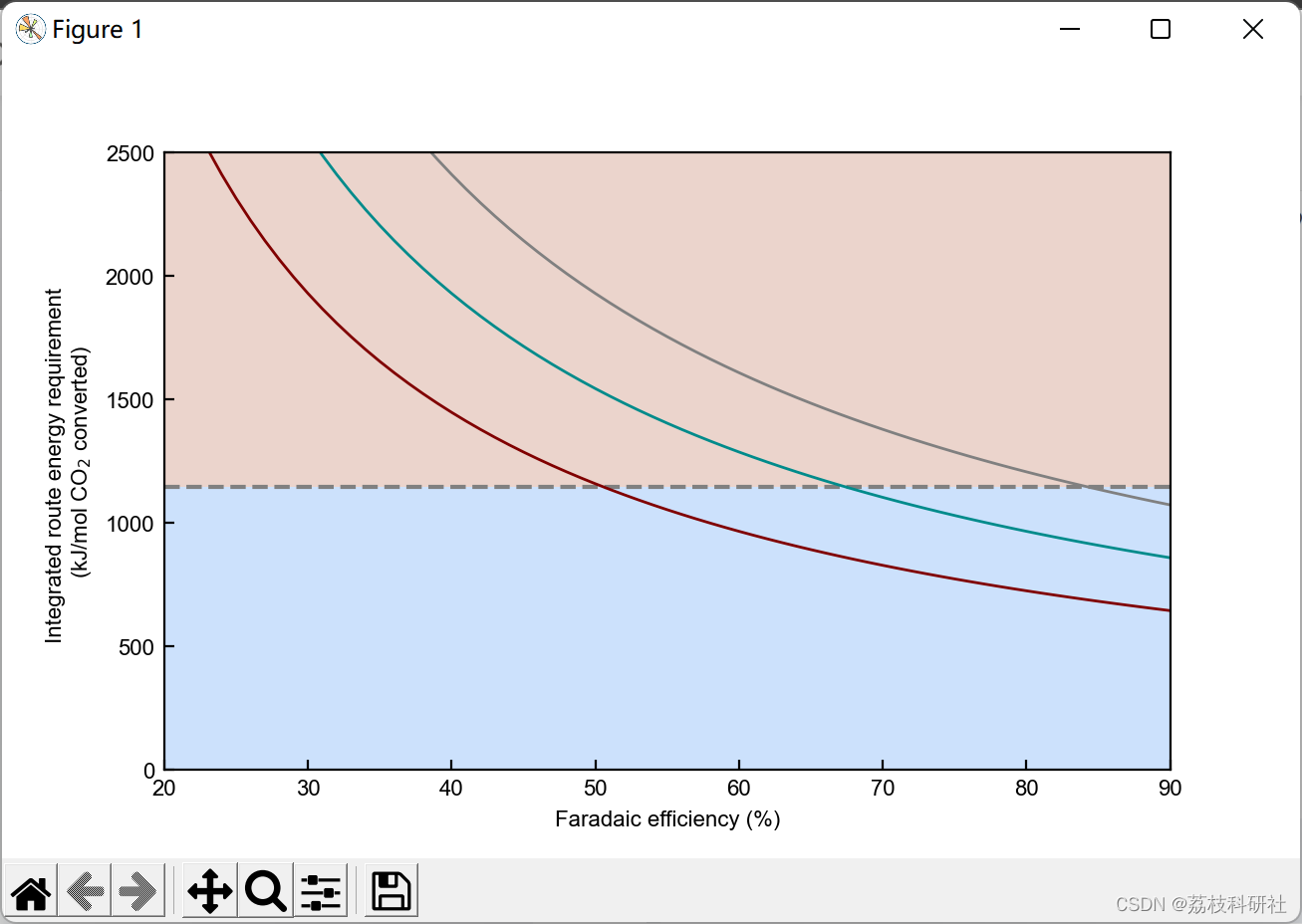
2.1 算例1

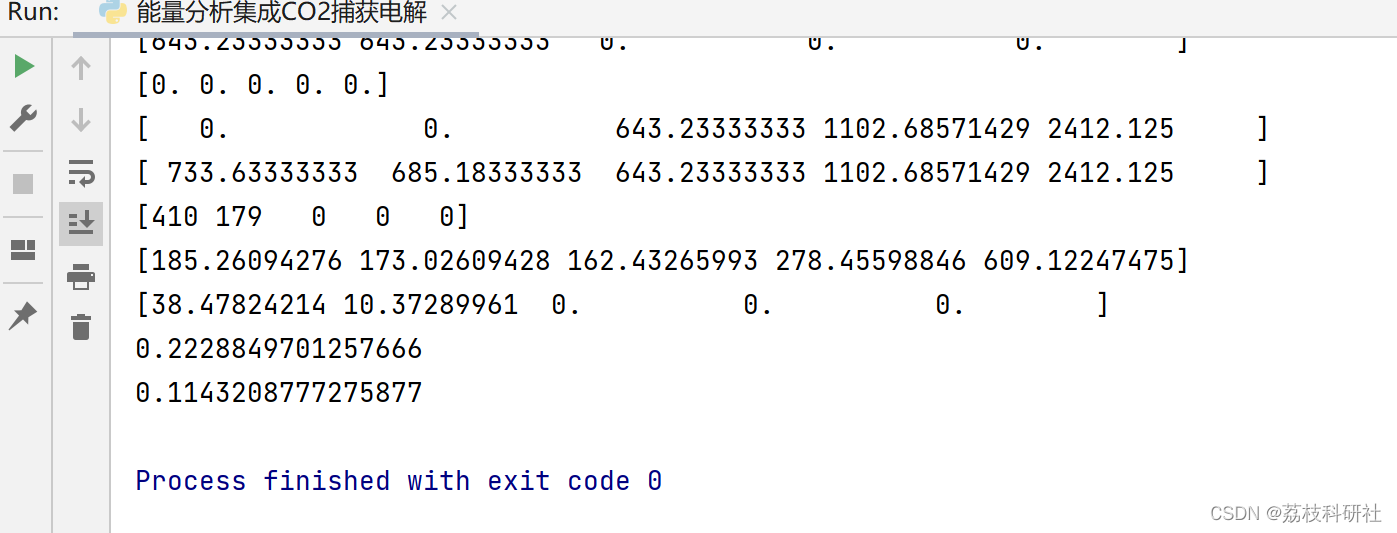
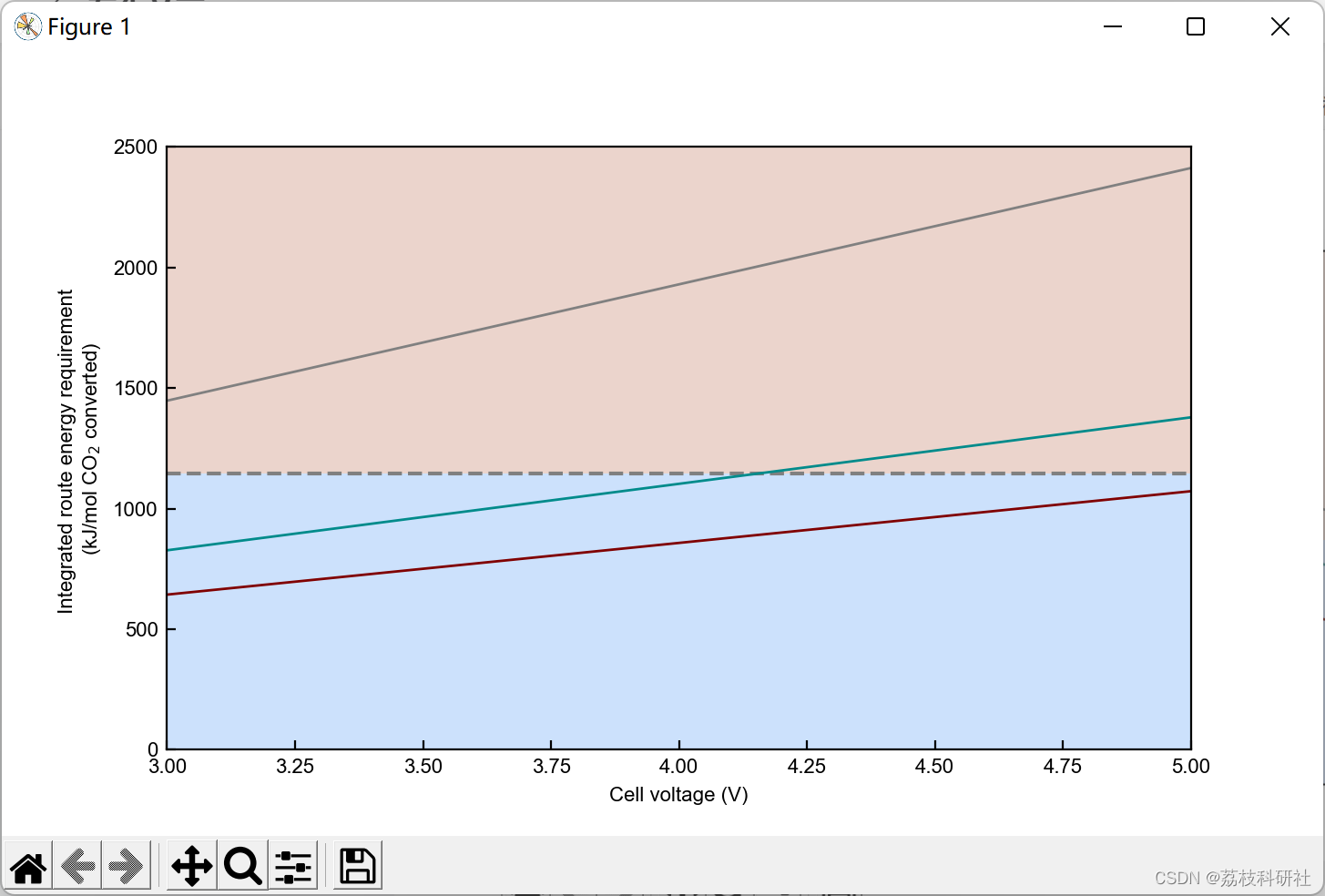
 2.2 算例2

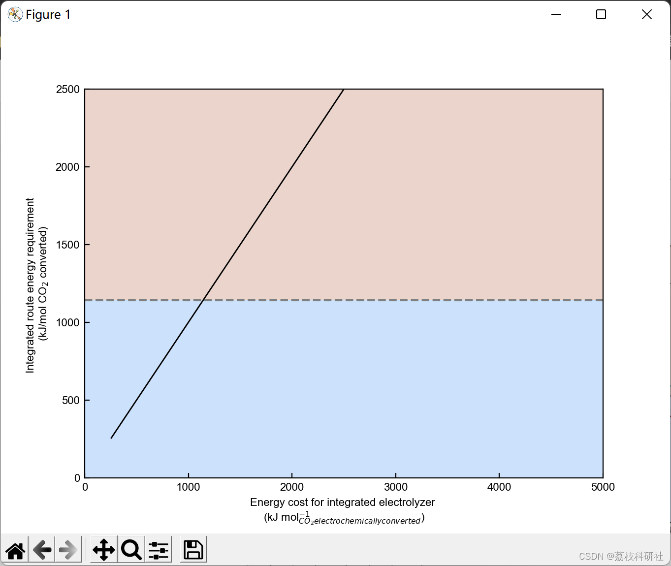
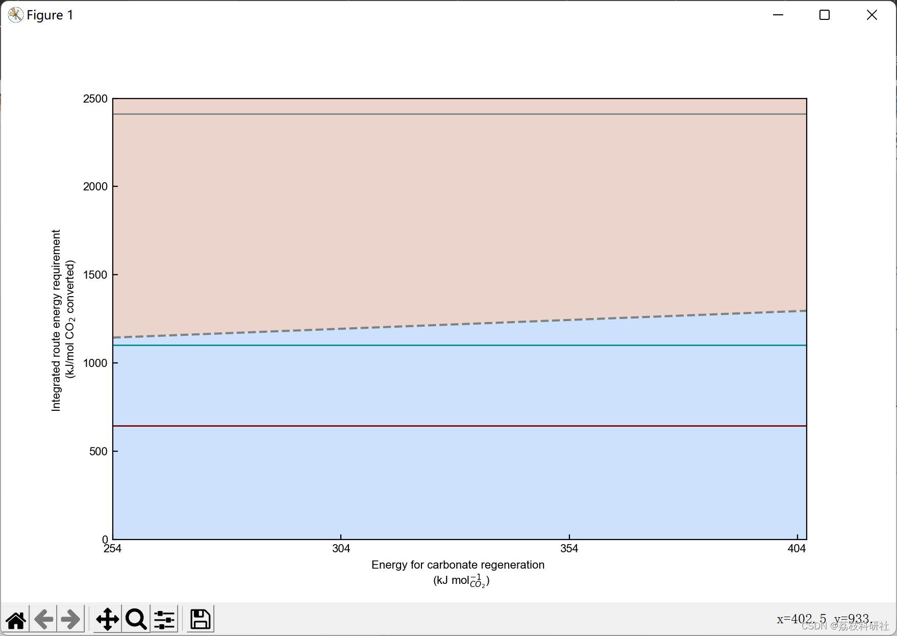
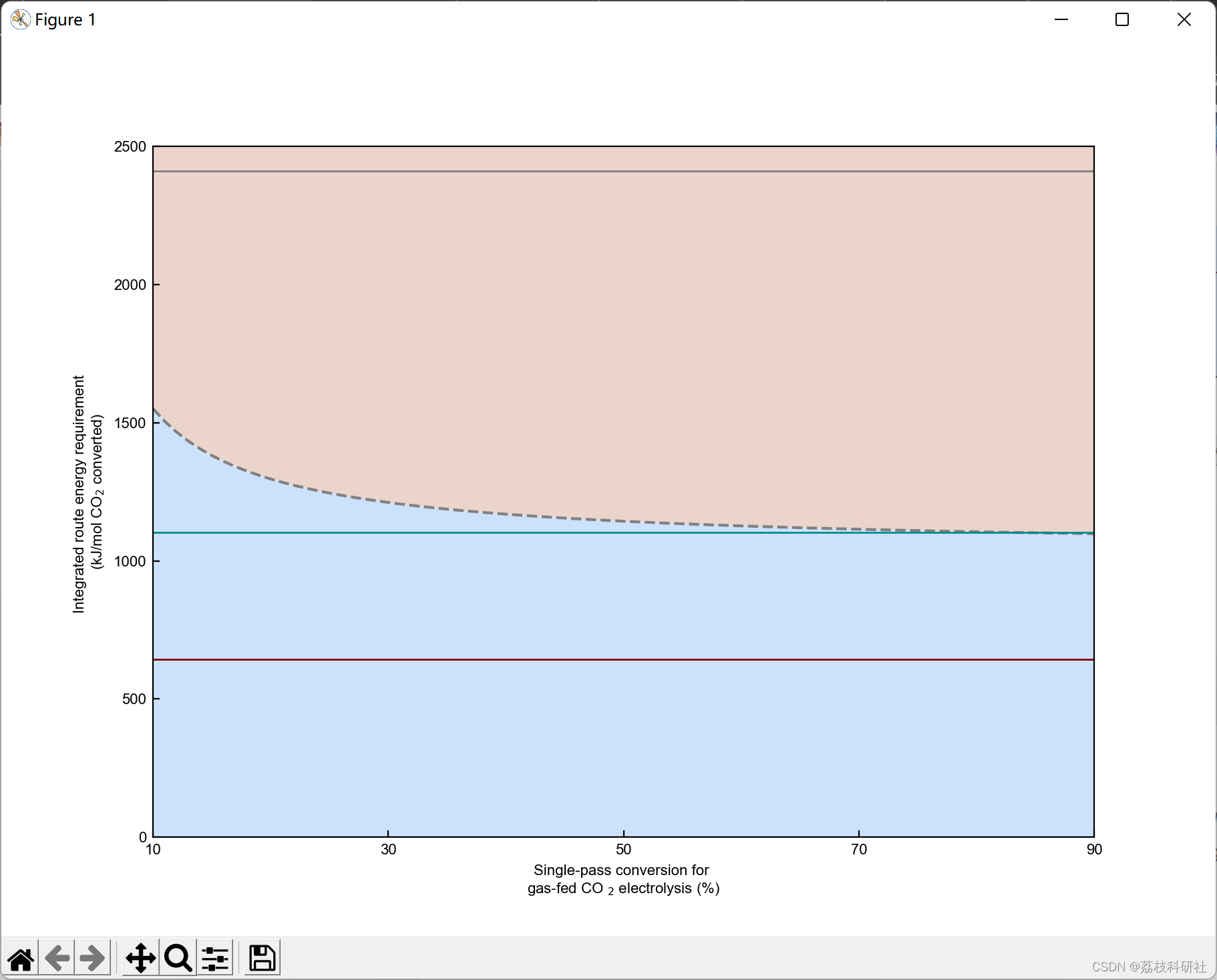
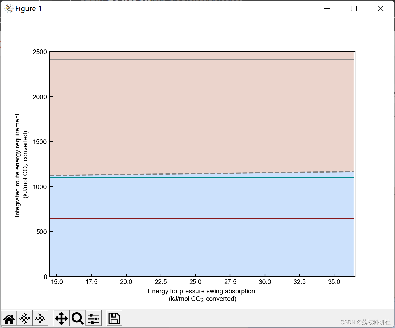
 2.3 算例3

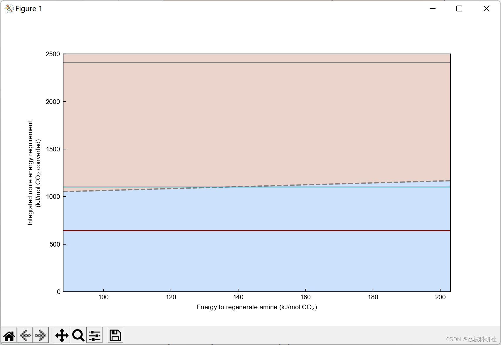
 2.4 算例4

部分代码：

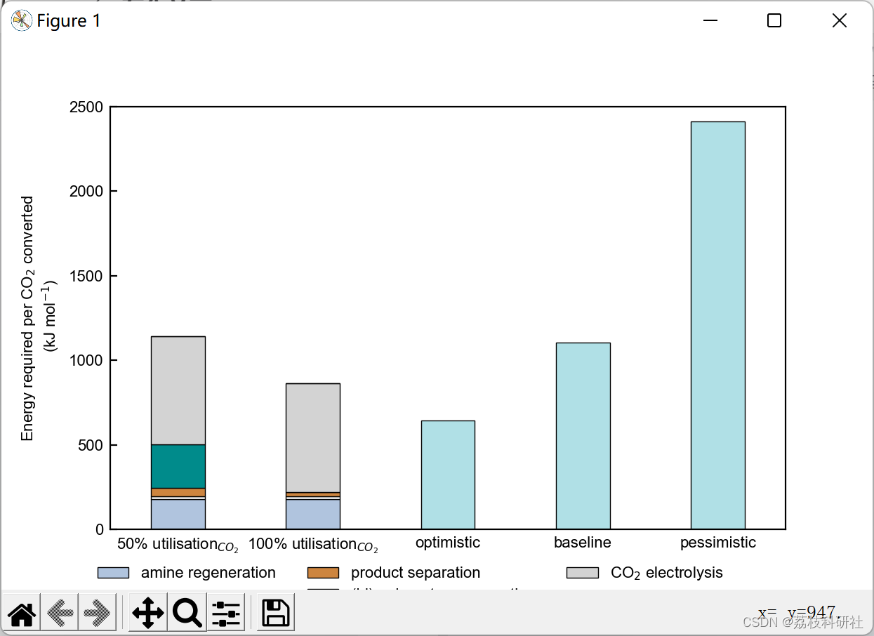
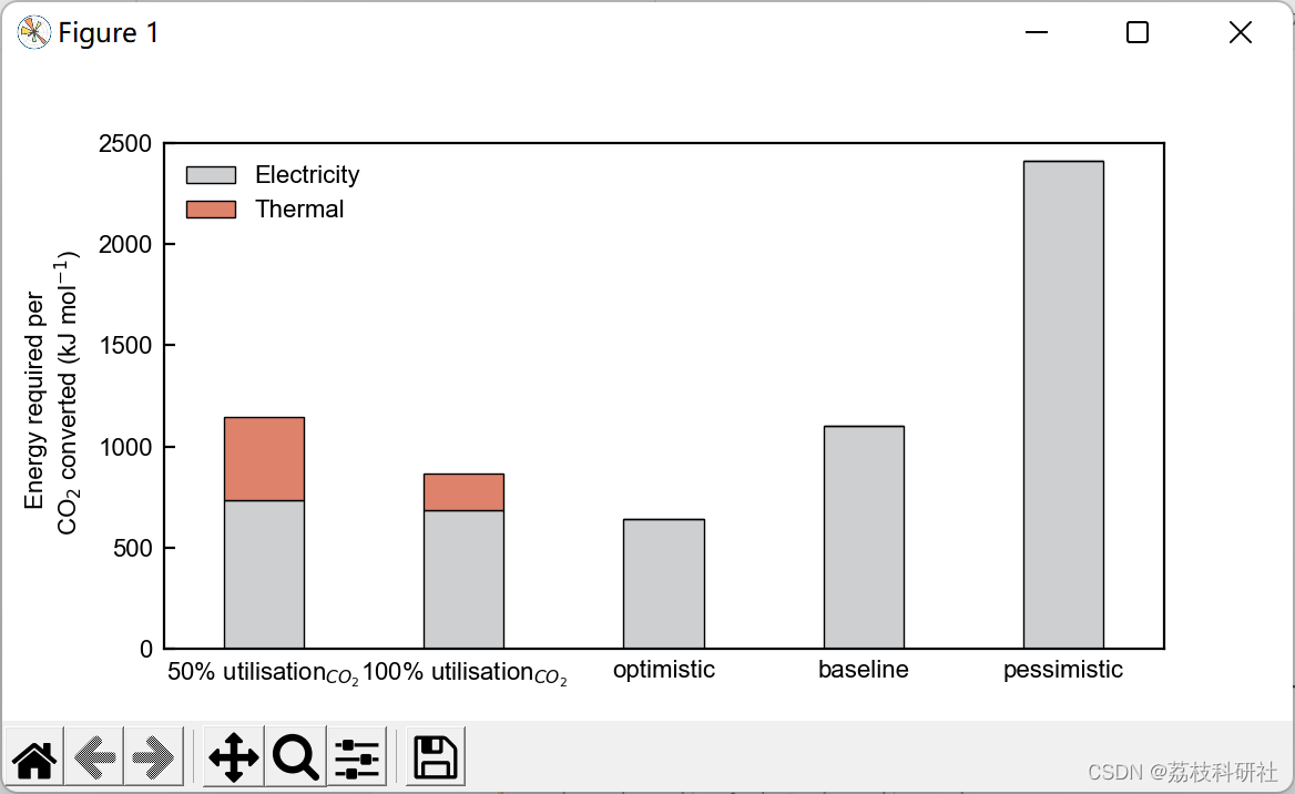
#Assuming the amine solution with salts has the same conductivity to 1 M KOH aq solution.
plt.rcParams['font.family']='Arial' #set font to be Arial
plt.rcParams['font.size']=8 #set font size to be 8
fig=plt.gcf()
fig.set_size_inches((2.33*4/3, 2.33)) #set figure size
ax= fig.add_subplot(111)
current=np.arange(-4, 305, 5) #define current densities from 1 to 300 mA cm-2
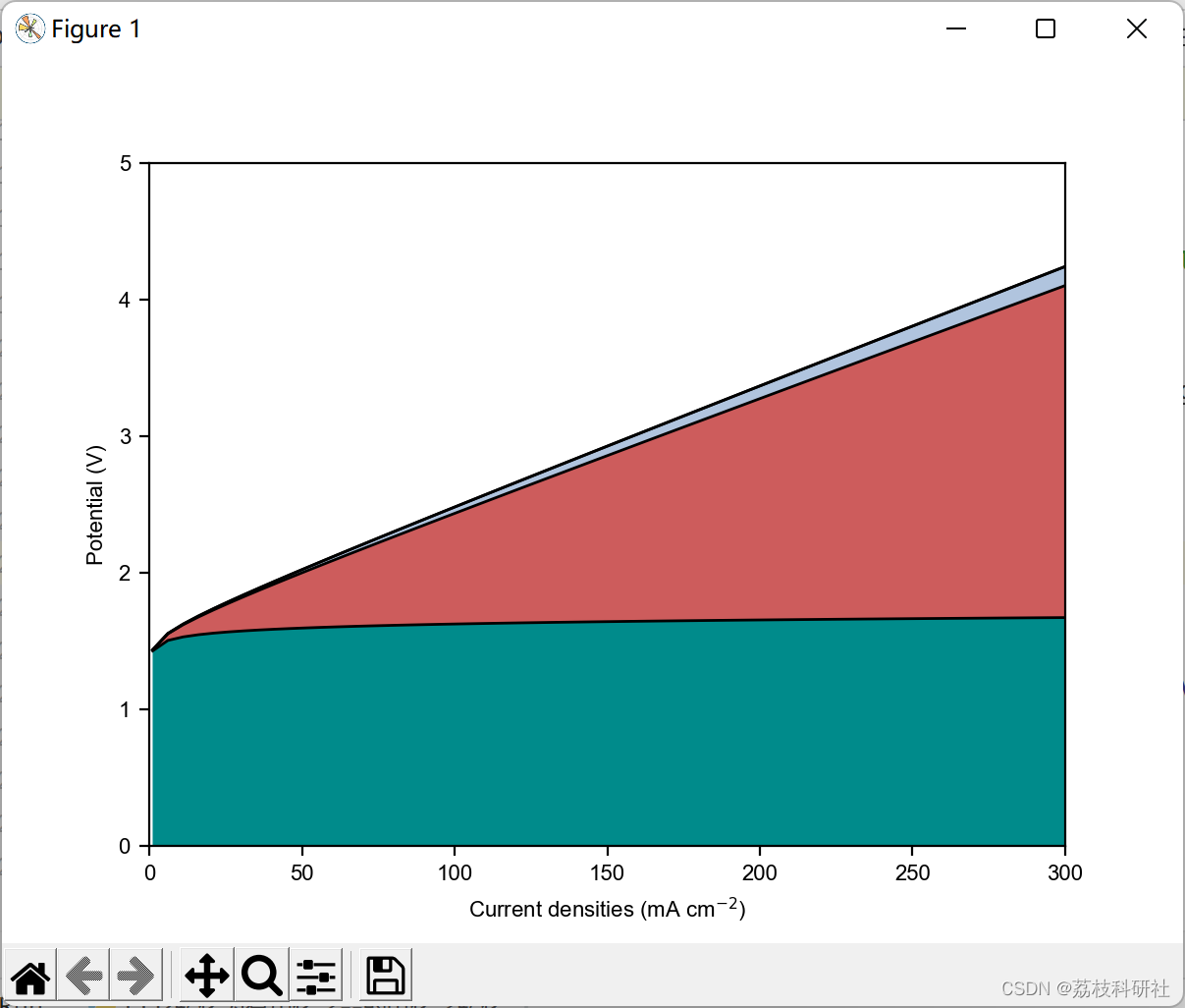
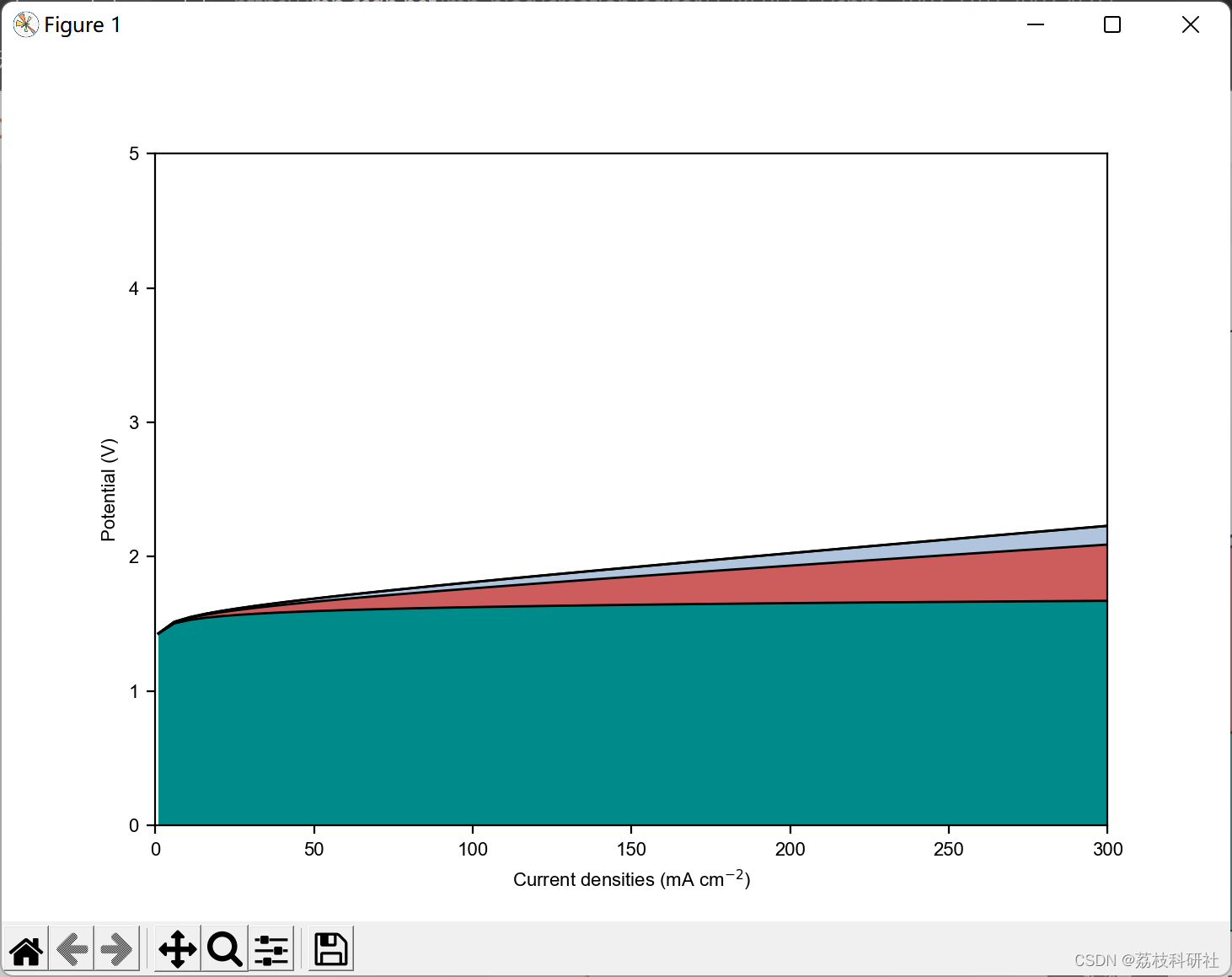
Eoer, Ememb, Eanolyte, Ecatholyte=estEwithsalts(current) #calculate the potential losses

plt.plot(current, Eoer, 'k', lw=1) #plot the anode potential loss
plt.plot(current, Ecatholyte+Eoer, 'k', lw=1) #plot ohmic loss from capture media
plt.plot(current, Eanolyte+Ecatholyte+Eoer, 'k', lw=1) #plot ohmic loss from anolyte
plt.plot(current, Ecatholyte+Eanolyte+Ememb+Eoer, 'k', lw=1) #plot ohmic loss from membrane

#Fill different colors to highlight the potential contributions
plt.fill_between(current, Eoer, 0, facecolor='darkcyan')
plt.fill_between(current, Eoer+Ecatholyte, Eoer, facecolor='indianred')
plt.fill_between(current, Eoer+Ecatholyte, Eoer+Ecatholyte, facecolor='r')
plt.fill_between(current, Eanolyte+Ecatholyte+Eoer, Eoer+Ecatholyte, facecolor='lightsteelblue')
plt.fill_between(current, Ecatholyte+Eanolyte+Ememb+Eoer, Eanolyte+Ecatholyte+Eoer, facecolor='firebrick')

plt.xlim(0,300) #set x-axis limits
plt.ylim(0,5) #set y-axis limits

plt.xlabel('Current densities (mA cm$^{-2}$)') #set xlabel
plt.ylabel('Potential (V)') #set ylabel
plt.show()
#fig.savefig('Figure/potentials breakup with inorganic salts.eps', bbox_inches='tight', pad_inches=0, transparent=True)


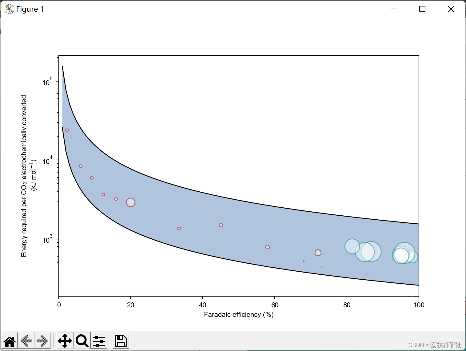
f=pd.read_excel('literature data.xlsx', sheet_name='Combine') #Read literature data of integrated electrolyzer in the excel spreadsheet
j_combine=f['Current densities'] #Read all the reported current densities of integrated electrolyzer, mA cm-2
fe_combine=f['FE(%) of CO']/100 #Read all the reported Faradaic efficiencies of the integrated electrolyzer
Ec_combine=f['Cathode Potential (V)'] #Read reported cathode potential, V
Eother_combine=estEother(j_combine) #Calculate the total potential except cathode potential from current densities
E_combine=-Ec_combine+Eother_combine #Calculate the cell potential
Q_combine=np.dot(E_combine, 2*96485)/(fe_combine*1000) #Calculate the energy cost of the integrated electrolyzers

ff=pd.read_excel('literature data.xlsx', sheet_name='Separate') #Read literature data of gas-fed electrolyzer in the excel spreadsheet
z = 2 #Number of charge transfered to produce one molecule of product
F = 96485 # A mol-1 Faraday constant
j_s=ff['Current densities'] #Read all the reported current densities of gas-fed electrolyzer, mA cm-2
E_s=ff['Calculated Cell Voltage (V) '] #Read all the reported cell potentials of the gas-fed electrolyzers
fe_s=ff['FE(%) of CO']/100 #Read all the reported Faradaic efficiencies of the gas-fed electrolyzer
Q_s=np.dot(E_s, z*F)/(fe_s*1000) #Calculate the energy cost of the gas-fed electrolyzers

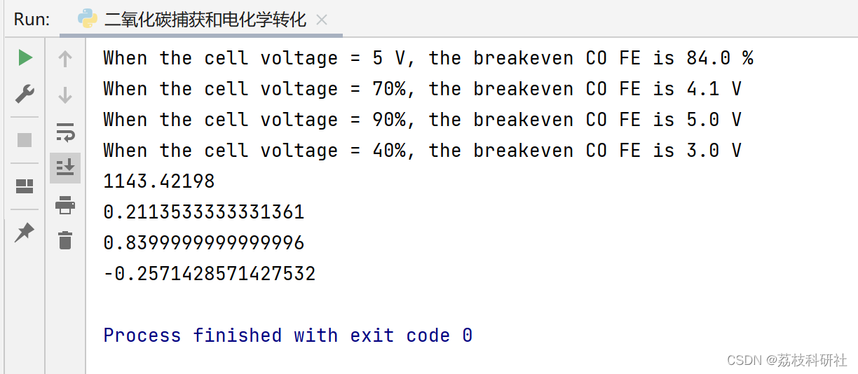
FE=np.arange(0.01,1.01,0.01) # Set a range of CO FE
E=np.arange(1.23+0.104,8,(8-1.23-0.104)/100) #Set a range of cell potentials
FEFE, EE = np.meshgrid(FE, E) #build a mesh grid of CO FE and cell potentials
Q=EE*z*F/FEFE/1000 #Calculate the energy cost of the electrolyzer using the mesh grid, kJ/molCO2 converted.

plt.rcParams['font.family']='Arial' #Set font to be Arial
plt.rcParams['font.size']=8 #Set fontsize to be 8
fig=plt.gcf()
fig.set_size_inches((2.33*4/3*1.5, 2.33*1.5)) #Set Figure size
ax= fig.add_subplot(111)

plt.plot(FE*100, Q.T[:,0],'k', lw=1) #Plot the lower limit
plt.plot(FE*100, Q.T[:,-1],'k',lw=1) #Plot the upper limit
#Highlight the region the electrolyzer will fall in.
plt.fill_between(FE*100, Q.T[:, 0], Q.T[:,-1], facecolor='lightsteelblue')
#Plot the energy performance of the integrated electrolyzers
plt.scatter(fe_combine[:-1]*100, Q_combine[:-1],
         s=j_combine[:-1].values, alpha=0.5,  facecolor='white', edgecolors='darkred')
#Plot the energy performance of the gas-fed electrolyzers
plt.scatter(fe_s*100, Q_s, s=j_s.values,  facecolor='w', alpha=0.5, edgecolors='darkcyan')

plt.xlim(0,100) #Set xaxis limits

plt.xlabel('Faradaic efficiency (%)') #Set xlabel
plt.ylabel('Energy required per CO$_2$ electrochemically converted \n (kJ mol$^{-1}$)') #Set ylabel

plt.yscale('log') #Set y-axis in log scale.
plt.show()
#fig.savefig('Figure/co2 electrolysis comparison.png', bbox_inches='tight', dpi=1200, pad_inches=0, transparent=True) #Save the figure.

🎉3 参考文献

部分理论来源于网络，如有侵权请联系删除。

[1]葛建邦. LiCl基熔盐体系中CO_2的捕获和电化学研究[D].北京科技大学,2017.

[2]Energy comparison of sequential and integrated CO2 capture and electrochemical conversion The contributing authors include Mengran Li, Erdem Irtem, Hugo Pieter Iglesias van Montfort, Maryam Abdinejad, Thomas Burdyny*

🌈4 Matlab代码实现