
mobileNetV1网络解析,以及实现(pytorch)
Google提出了移动端模型MobileNet,其核心是采用了深度可分离卷积,其不仅可以降低模型计算复杂度,而且可以大大降低模型大小,适合应用在真实的移动端应用场景。在认识MobileNet之前,我们先了解一下什么是深度可分离卷积,以及和普通卷积的区别。
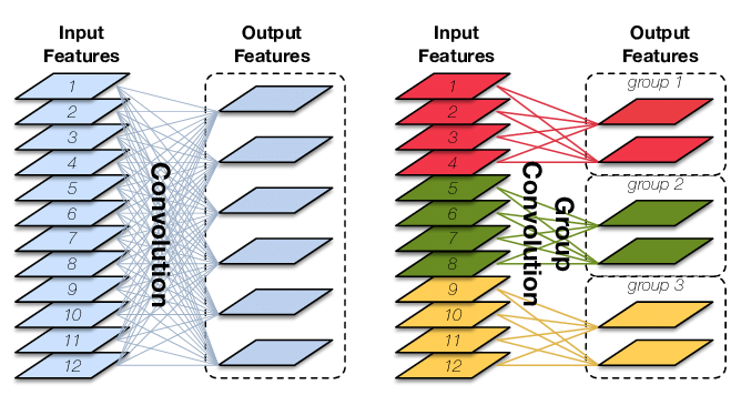
上面的图片展示了普通卷积和分组卷积的不同,下面我们通过具体的例子来看。
普通卷积
标准卷积运算量的计算公式:
F
L
O
P
s
=
(
2
×
C
0
×
K
2
−
1
)
×
H
×
W
×
C
1
{FLOPs }=\left(2 \times C_{0} \times K^{2}-1\right) \times H \times W \times C_{1}
FLOPs=(2×C0×K2−1)×H×W×C1
计算公式参考:深度学习之(经典)卷积层计算量以及参数量总结 (考虑有无bias,乘加情况) - 琴影 - 博客园 (cnblogs.com)
参数量计算公式: K 2 × C 0 × C 1 K^{2} \times C_{0} \times C{1} K2×C0×C1
C 0 C_{0} C0 :输入的通道。
K:卷积核大小。
H,W:输出 feature map的大小
C 1 C_{1} C1:输出通道的大小。
bias=False,即不考虑偏置的情况有-1,有True时没有-1。
举例:
输入的尺寸是227×227×3,卷积核大小是11×11,输出是6,输出维度是55×55,
我们带入公式可以计算出
参数量:
1 1 2 × 3 × 6 11^2 \times 3 \times 6 112×3×6=2178
运算量:
2 × 3 × 1 1 2 × 55 × 55 × 6 2 \times 3 \times11^{2}\times 55\times 55 \times 6 2×3×112×55×55×6=13176900
分组卷积
分组卷积则是对输入feature map进行分组,然后每组分别卷积。
假设输入feature map的尺寸仍为 C 0 × H × W C_{0}\times H \times W C0×H×W,输出feature map的数量为 C 1 C_{1} C1个,如果设定要分成G个groups,则每组的输入feature map数量为 C 0 G \frac{C_{0}}{G} GC0,每组的输出feature map数量为 C 1 G \frac{C{1}}{G} GC1,每个卷积核的尺寸为 C 0 G × K × K \frac{C_{0}}{G}\times K \times K GC0×K×K,卷积核的总数仍为 C 1 C_{1} C1个,每组的卷积核数量为 C 1 G \frac{C{1}}{G} GC1,卷积核只与其同组的输入map进行卷积,卷积核的总参数量为 N × C 0 G × K × K N\times \frac{C_{0}}{G}\times K \times K N×GC0×K×K,总参数量减少为原来的 1 G \frac{1}{G} G1。
计算量公式:
[
(
2
×
K
2
×
C
0
/
g
+
1
)
×
H
×
W
×
C
o
/
g
]
×
g
\left[\left(2 \times K^{2} \times C_{0} / g +1\right) \times H \times W \times C_{o} / g\right] \times g
[(2×K2×C0/g+1)×H×W×Co/g]×g
分组卷积的参数量为:
K
∗
K
∗
C
0
g
∗
C
1
g
∗
g
K * K * \frac{C_{0}}{g} * \frac{C_{1}}{g} * g
K∗K∗gC0∗gC1∗g
举例:
输入的尺寸是227×227×3,卷积核大小是11×11,输出是6,输出维度是55×55,group为3
我们带入公式可以计算出
参数量:
1 1 2 × 3 3 × 6 3 × 3 11^2 \times \frac{3}{3} \times \frac{6}{3} \times 3 112×33×36×3=726
运算量:
[ ( 2 × 1 1 2 × 3 / 3 + 1 ) × 55 × 55 × 6 / 3 ] × 3 \left[\left(2 \times 11^{2} \times3 / 3 +1\right) \times 55 \times 55 \times 6 / 3\right] \times 3 [(2×112×3/3+1)×55×55×6/3]×3=2205225
深度可分离卷积(Depthwise separable conv)
设输入特征维度为 D F × D F × M D_{F}\times D_{F}\times M DF×DF×M,M为通道数, D k D_{k} Dk为卷积核大小,M为输入的通道数, N为输出的通道数,G为分组数。
当分组数量等于输入map数量,输出map数量也等于输入map数量,即M=N=G,N个卷积核每个尺寸为$D_{k}\times D_{k}\times 1 $时,Group Convolution就成了Depthwise Convolution。
逐点卷积就是把G组卷积用conv1x1拼接起来。如下图:

深度可分离卷积有深度卷积+逐点卷积。计算如下:
-
深度卷积:设输入特征维度为 D F × D F × M D_{F}\times D_{F}\times M DF×DF×M,M为通道数。卷积核的参数为 D k × D k × 1 × M D_{k}\times D_{k}\times 1 \times M Dk×Dk×1×M。输出深度卷积后的特征维度为: D F × D F × M D_{F}\times D_{F}\times M DF×DF×M。卷积时每个通道只对应一个卷积核(扫描深度为1),所以 FLOPs为: M × D F × D F × D K × D K M\times D_{F}\times D_{F}\times D_{K}\times D_{K} M×DF×DF×DK×DK
-
逐点卷积:输入为深度卷积后的特征,维度为 D F × D F × M D_{F}\times D_{F}\times M DF×DF×M。卷积核参数为 1 × 1 × M × N 1\times1\times M\times N 1×1×M×N。输出维度为 D F × D F × N D_{F}\times D_{F}\times N DF×DF×N。卷积过程中对每个特征做 1 × 1 1 \times 1 1×1的标准卷积, FLOPs为: N × D F × D F × M N \times D_{F} \times D_{F}\times M N×DF×DF×M
将上面两个参数量相加就是 D k × D k × M + M × N D_{k} \times D_{k} \times M+M \times N Dk×Dk×M+M×N
所以深度可分离卷积参数量是标准卷积的 D K × D K × M + M × N D K × D K × M × N = 1 N + 1 D K 2 \frac{D_{K} \times D_{K} \times M+M \times N}{D_{K} \times D_{K} \times M \times N}=\frac{1}{N}+\frac{1}{D_{K}^{2}} DK×DK×M×NDK×DK×M+M×N=N1+DK21
mobileNetV1
详见论文翻译:
https://blog.csdn.net/hhhhhhhhhhwwwwwwwwww/article/details/122692846
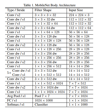
mobileNetV1的网络结构如下图.前面的卷积层中除了第一层为标准卷积层外,其他都是深度可分离卷积(Conv dw + Conv/s1),卷积后接了一个7*7的平均池化层,之后通过全连接层,最后利用Softmax激活函数将全连接层输出归一化到0-1的一个概率值,根据概率值的高低可以得到图像的分类情况。
pytorch版本
import torch
import torch.nn as nn
import torchvision

def BottleneckV1(in_channels, out_channels, stride):
  return  nn.Sequential(
        nn.Conv2d(in_channels=in_channels,out_channels=in_channels,kernel_size=3,stride=stride,padding=1,groups=in_channels),
        nn.BatchNorm2d(in_channels),
        nn.ReLU6(inplace=True),
        nn.Conv2d(in_channels=in_channels, out_channels=out_channels, kernel_size=1, stride=1),
        nn.BatchNorm2d(out_channels),
        nn.ReLU6(inplace=True)
    )

class MobileNetV1(nn.Module):
    def __init__(self, num_classes=1000):
        super(MobileNetV1, self).__init__()

        self.first_conv = nn.Sequential(
            nn.Conv2d(in_channels=3,out_channels=32,kernel_size=3,stride=2,padding=1),
            nn.BatchNorm2d(32),
            nn.ReLU6(inplace=True),
        )

        self.bottleneck = nn.Sequential(
            BottleneckV1(32, 64, stride=1),
            BottleneckV1(64, 128, stride=2),
            BottleneckV1(128, 128, stride=1),
            BottleneckV1(128, 256, stride=2),
            BottleneckV1(256, 256, stride=1),
            BottleneckV1(256, 512, stride=2),
            BottleneckV1(512, 512, stride=1),
            BottleneckV1(512, 512, stride=1),
            BottleneckV1(512, 512, stride=1),
            BottleneckV1(512, 512, stride=1),
            BottleneckV1(512, 512, stride=1),
            BottleneckV1(512, 1024, stride=2),
            BottleneckV1(1024, 1024, stride=1),
        )

        self.avg_pool = nn.AvgPool2d(kernel_size=7,stride=1)
        self.linear = nn.Linear(in_features=1024,out_features=num_classes)
        self.dropout = nn.Dropout(p=0.2)
        self.softmax = nn.Softmax(dim=1)

        self.init_params()

    def init_params(self):
        for m in self.modules():
            if isinstance(m, nn.Conv2d):
                nn.init.kaiming_normal_(m.weight)
                nn.init.constant_(m.bias,0)
            elif isinstance(m, nn.Linear) or isinstance(m, nn.BatchNorm2d):
                nn.init.constant_(m.weight, 1)
                nn.init.constant_(m.bias, 0)

    def forward(self, x):
        x = self.first_conv(x)
        x = self.bottleneck(x)
        x = self.avg_pool(x)
        x = x.view(x.size(0),-1)
        x = self.dropout(x)
        x = self.linear(x)
        out = self.softmax(x)
        return out

if __name__=='__main__':
    model = MobileNetV1()
    print(model)

    input = torch.randn(1, 3, 224, 224)
    out = model(input)
    print(out.shape)
相关文章
- Android系列之网络(二)----HTTP请求头与响应头
- Android代码优化----PullToRefresh+universal-image-loader实现从网络获取数据并刷新
- Android网络开发之WebKet引擎基础
- JZ2440 启动NFS网络文件系统_初试led驱动
- 网络爬虫简介
- Android kotlin 进阶之用Retrofit+OkHttp+协程+LiveData搭建MVVM来实现网络请求(网络数据JSON解析)显示在RecyclerView
- Java IO:操作系统的IO处理过程以及5种网络IO模型
- [网络]_获取内外网IP地址【Auto.js】
- pytorch手写数字识别验证四流网络
- jittor和pytorch生成网络对比之wgan_gp
- jittor和pytorch生成网络对比之gan
- jittor和pytorch生成网络对比之cyclegan
- jittor和pytorch生成网络对比之began
- pytorch定义神经卷积网络CNN源码
- pytorch生成网络WGAN-GP实例
- pytorch 之手写数字生成网络
- PyTorch 实现孪生网络识别面部相似度
- 干货下载:可能是你见过的最全的网络爬虫总结
- PyTorch下的网络可视化方式和工具
- 【pytorch】named_parameters()、parameters()、state_dict()==>给出网络的名字和参数的迭代器
- ios学习网络------4 UIWebView以三种方式中的本地数据
- 《Kubernetes网络权威指南》读书笔记 | 岂止iptables:Kubernetes Service官方实现细节探秘
- Pytorch网络模型转Onnx格式,多种方法(opencv、onnxruntime、c++)调用Onnx
- 嵌入式linux开发,tcpdump移植,tcpdump网络数据抓包工具移植
- 还在谈论云计算吗?算力网络来啦!!!
- RK3399平台开发系列讲解(网络篇)7.5、图解HTTP
- C++搭建集群聊天室(六):muduo网络库