【数据分析】大型ADCP数据集的处理和分析（Matlab代码实现）

 👨‍🎓个人主页：研学社的博客 

💥💥💞💞欢迎来到本博客❤️❤️💥💥

🏆博主优势：🌞🌞🌞博客内容尽量做到思维缜密，逻辑清晰，为了方便读者。

⛳️座右铭：行百里者，半于九十。

📋📋📋本文目录如下：🎁🎁🎁

目录

💥1 概述

📚2 运行结果

🌈3 Matlab代码实现

🎉4 参考文献

---

💥1 概述

本文将指导您完成处理和分析船载（VM-ADCP）和降低声学多普勒电流轮廓仪（L-ADCP）所需的步骤。

📚2 运行结果

主函数部分代码：

clc;clear;
 
% Set coefficients
eta0=0.01; % highest height of eddy
R=300; % eddy's radius
f=0.01; % coriolis coefficient
g=9.81; % gravity constant
 
% Set grid
x=-500:10:500;
y=-500:10:500;
[x y]=meshgrid(x,y);
 
% Set sea surface height
eta=eta0*exp(-(x.^2+y.^2)/R^2);
 
% Calcualte geostrophic velocity
v=(g*eta0)/f*(-2*x/R^2).*exp(-(x.^2+y.^2)/R^2);
u=-(g*eta0)/f*(-2*y/R^2).*exp(-(x.^2+y.^2)/R^2);

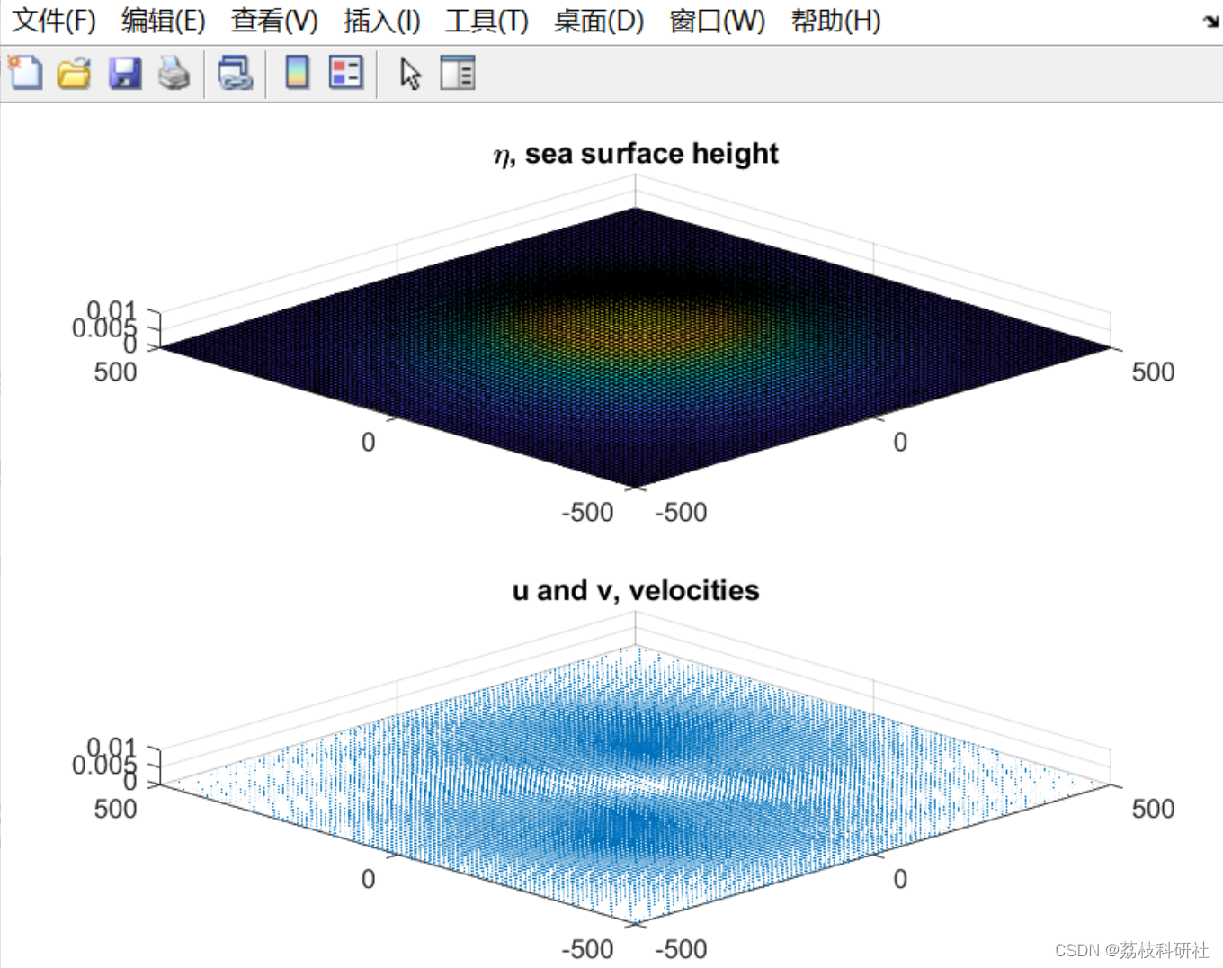
% Visualization
figure(1)
clf
set(gcf,'color','w')
subplot(2,1,1)
surf(x,y,eta)
view([-45 80])
title('\eta, sea surface height','fontweight','bold')
subplot(2,1,2)
z0=zeros(size(x));
quiver3(x,y,z0,u,v,z0)
view([-45 80])
axis([-500 500 -500 500 0 0.01])
title('u and v, velocities','fontweight','bold')

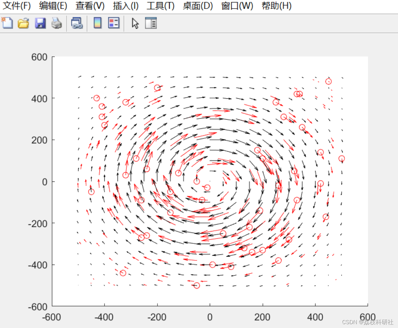
%% get observations

n_obs=200;

x_vec=x(:);
y_vec=y(:);
u_vec=u(:);
v_vec=v(:);

ixr=randi(numel(x_vec),[n_obs,1]);
x_obs=x_vec(ixr);
y_obs=y_vec(ixr);
u_obs=u_vec(ixr);
v_obs=v_vec(ixr);

figure(2)
clf
hold on
quiver(x,y,u,v,'k')
quiver(x_obs,y_obs,u_obs,v_obs,'r')

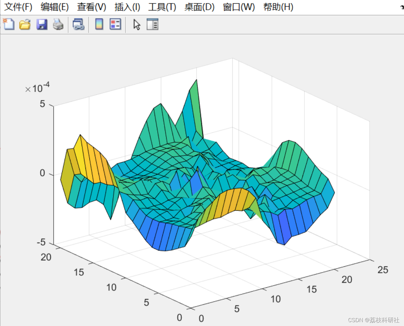
figure(3)
clf
div=divergence(u,v);
surf(div)
shading flat

🌈3 Matlab代码实现

🎉4 参考文献

部分理论来源于网络，如有侵权请联系删除。

[1]杨远征,徐超,李莎,何云开.2009-2012年南海海洋断面科学考察走航ADCP海流观测数据集[J].中国科学数据(中英文网络版),2019,4(03):152-161.