脉冲信号研究（matlab代码实现）

 👨‍🎓个人主页：研学社的博客 

💥💥💞💞欢迎来到本博客❤️❤️💥💥

🏆博主优势：🌞🌞🌞博客内容尽量做到思维缜密，逻辑清晰，为了方便读者。

⛳️座右铭：行百里者，半于九十。

📋📋📋本文目录如下：🎁🎁🎁

目录

💥1 概述

📚2 运行结果

🎉3 参考文献

🌈4 Matlab代码实现

---

💥1 概述

我们把脉冲信号从低电压到高电压的沿称为上升沿，从高电压到低电压的沿称为下降沿，有些数据也称为前沿和后沿。低电压叫低电平，高电压叫高电平。

假设脉冲信号的周期为t，脉冲宽度为t1，有一些基本概念如下。

f：指脉冲信号周期在一秒内变化的次数，即f = 1/T的周期越小，频率越大。

有了频率的概念，我们现在来讨论从PLC输入端输入的开关信号的最高频率。根据上一章关于扫描和PLC滞后的知识，PLC的扫描周期主要由用户程序的长度决定。假设扫描周期为20毫秒，考虑到输入滤波器的响应延迟为10毫秒，PLC的扫描周期为30毫秒。如果输入信号的变化小于30毫秒，从扫描原理可知，PLC可能检测不完全，也就是说输入信号的脉冲宽度必须大于30毫秒，所以输入信号的频率是有限的。

📚2 运行结果

 主函数代码：

clc
clear
close all
SampFreq=10000;
load impulse.mat
T = 0.08; % Time duration
Nt = length(impulse);% The number of samples in time domain
Nf = floor(Nt/2)+1;% The number of samples in frequency domain
f = (0 : Nf-1)/T; % frequency variables
t = (0 : Nt-1)/SampFreq;  % time variables

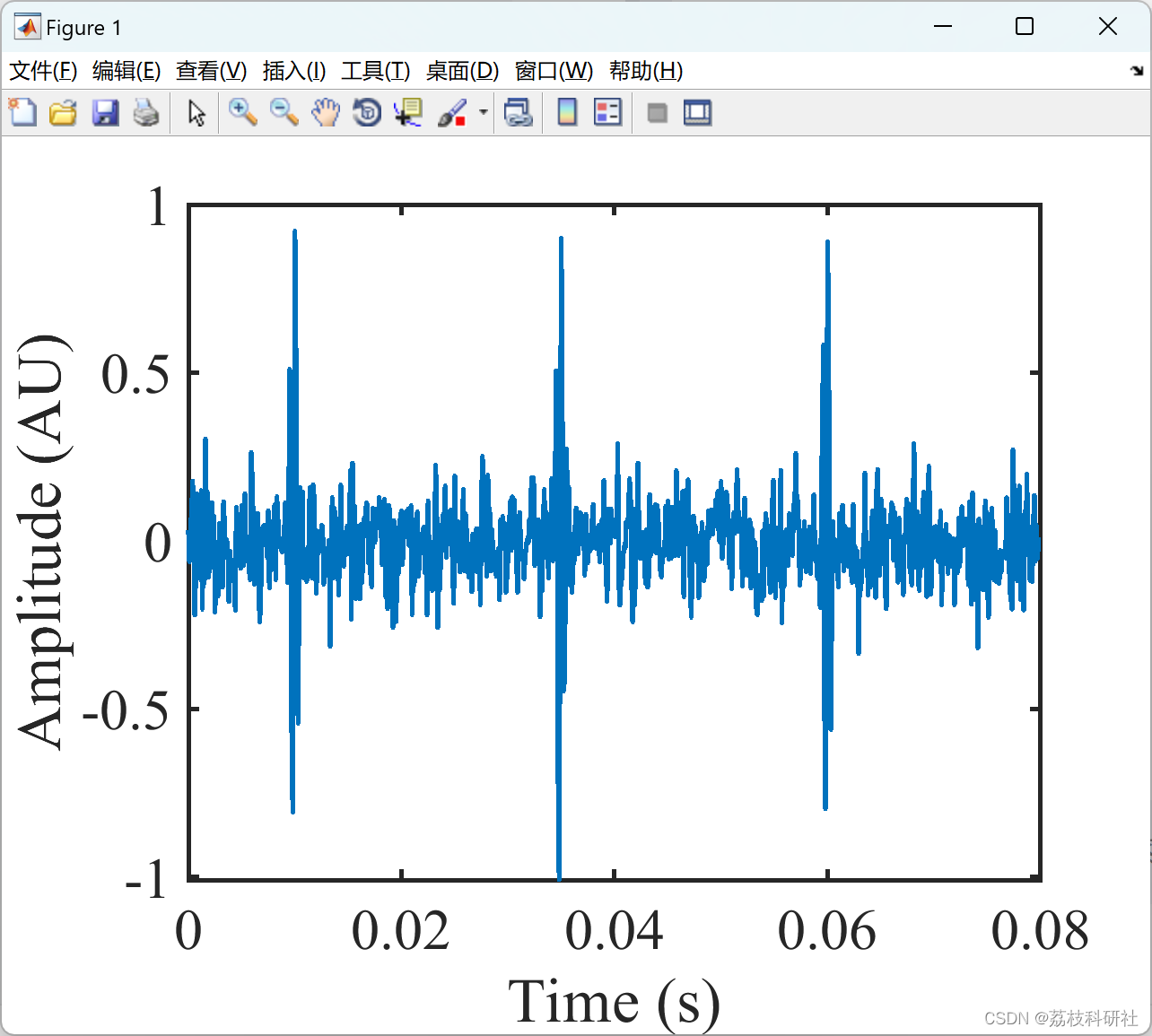
Sign = awgn(impulse,0,'measured');

figure
set(gcf,'Position',[20 100 640 500]);        
set(gcf,'Color','w'); 
plot(t,Sign,'linewidth',2);
xlabel('Time (s)','FontSize',24,'FontName','Times New Roman');
ylabel('Amplitude (AU)','FontSize',24,'FontName','Times New Roman');
set(gca,'FontSize',24)
set(gca,'linewidth',2);
set(gca,'FontName','Times New Roman')

fftspec = fft(Sign); % Obtain frequency-domain data of the signal
Dsn = fftspec(1:Nf); 
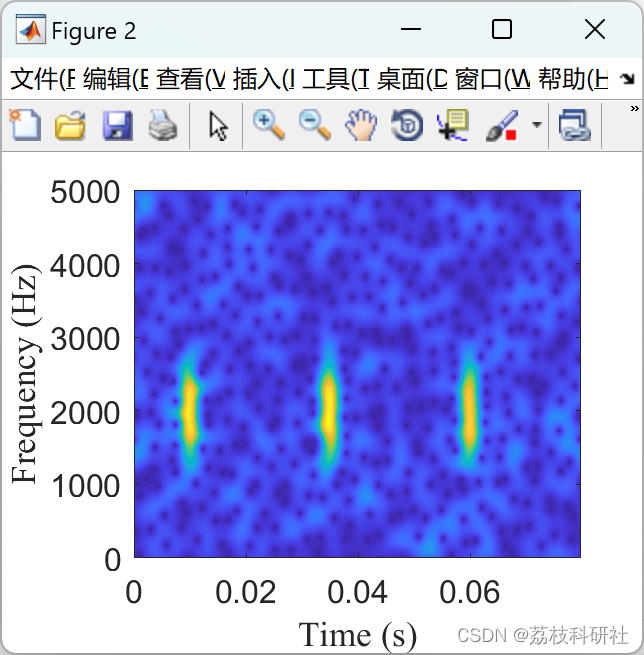
%% SFFT
Nfrebin = 1024;
window = 64;
figure
[Spec,f] = SFFT(Dsn(:),SampFreq,Nfrebin,window);
imagesc(t,f,abs(Spec));  
axis([0 max(t) 0 SampFreq/2]);
set(gcf,'Position',[20 100 320 250]);
set(gcf,'Color','w');    
xlabel('Time (s)','FontSize',12,'FontName','Times New Roman');
ylabel('Frequency (Hz)','FontSize',12,'FontName','Times New Roman');
set(gca,'YDir','normal')
set(gca,'FontSize',12);

%% Parameter setting
beta = 1e-8;  % this parameter can be smaller which will be helpful for the convergence, but it may cannot properly track fast varying GDs
alpha = 3e-7;  % if this parameter is larger, it will help the algorithm to find correct modes even the initial GDs are too rough. But it will introduce more noise and also may increase the interference between the signal modes
tol = 1e-8;
%% Mode 1 extraction
Envelope = abs(hilbert(Sign)); % envelope signal of the impulse signal
[~,tindex1] = max(Envelope);
peakenv1 = t(tindex1); % GD initialization by finding peak time of the envelope signal
iniGD1 = peakenv1*ones(1,length(Dsn)); % initial GD vector
[eGDest1 temp1] = GDMD(Dsn,T,iniGD1,alpha,beta,tol); % extract the signal mode
Desest1 = temp1(1,:,end);
DFs1 = [Desest1,conj(fliplr(Desest1(2:ceil(Nt/2))))]; eM1 = real(ifft(DFs1)); %Obtain the time-domain signal by inverse FFT; DFs1 denotes the bilateral spectrums
%% Mode 2 extraction
Dsresidue1 = Dsn - Desest1; % obtain the residual signal by removing the extracted component from the raw signal (in frequency domain)
residue1 = Sign - eM1; % Residual signal in time domain
reEnvelope1 = abs(hilbert(residue1)); % envelope signal of the residual signal
[~,tindex2] = max(reEnvelope1);
peakenv2 = t(tindex2); % GD initialization by finding peak time of the envelope signal
iniGD2 = peakenv2*ones(1,length(Dsn)); % initial GD vector
[eGDest2 temp2] = GDMD(Dsresidue1,T,iniGD2,alpha,beta,tol); % extract the signal mode
Desest2 = temp2(1,:,end);
DFs2 = [Desest2,conj(fliplr(Desest2(2:ceil(Nt/2))))]; eM2 = real(ifft(DFs2)); %Obtain the time-domain signal by inverse FFT;
%% Mode 3 extraction
Dsresidue2 = Dsresidue1 - Desest2; % obtain the residual signal by removing the extracted component from the raw signal (in frequency domain)
residue2 = residue1 - eM2; % Residual signal in time domain
reEnvelope2 = abs(hilbert(residue2)); % envelope signal of the residual signal
[~,tindex3] = max(reEnvelope2);
peakenv3 = t(tindex3); % GD initialization by finding peak time of the envelope signal
iniGD3 = peakenv3*ones(1,length(Dsn)); % initial GD vector
[eGDest3 temp3] = GDMD(Dsresidue2,T,iniGD3,alpha,beta,tol); % extract the signal mode
Desest3 = temp3(1,:,end);
DFs3 = [Desest3,conj(fliplr(Desest3(2:ceil(Nt/2))))]; eM3 = real(ifft(DFs3)); %Obtain the time-domain signal by inverse FFT;
%%

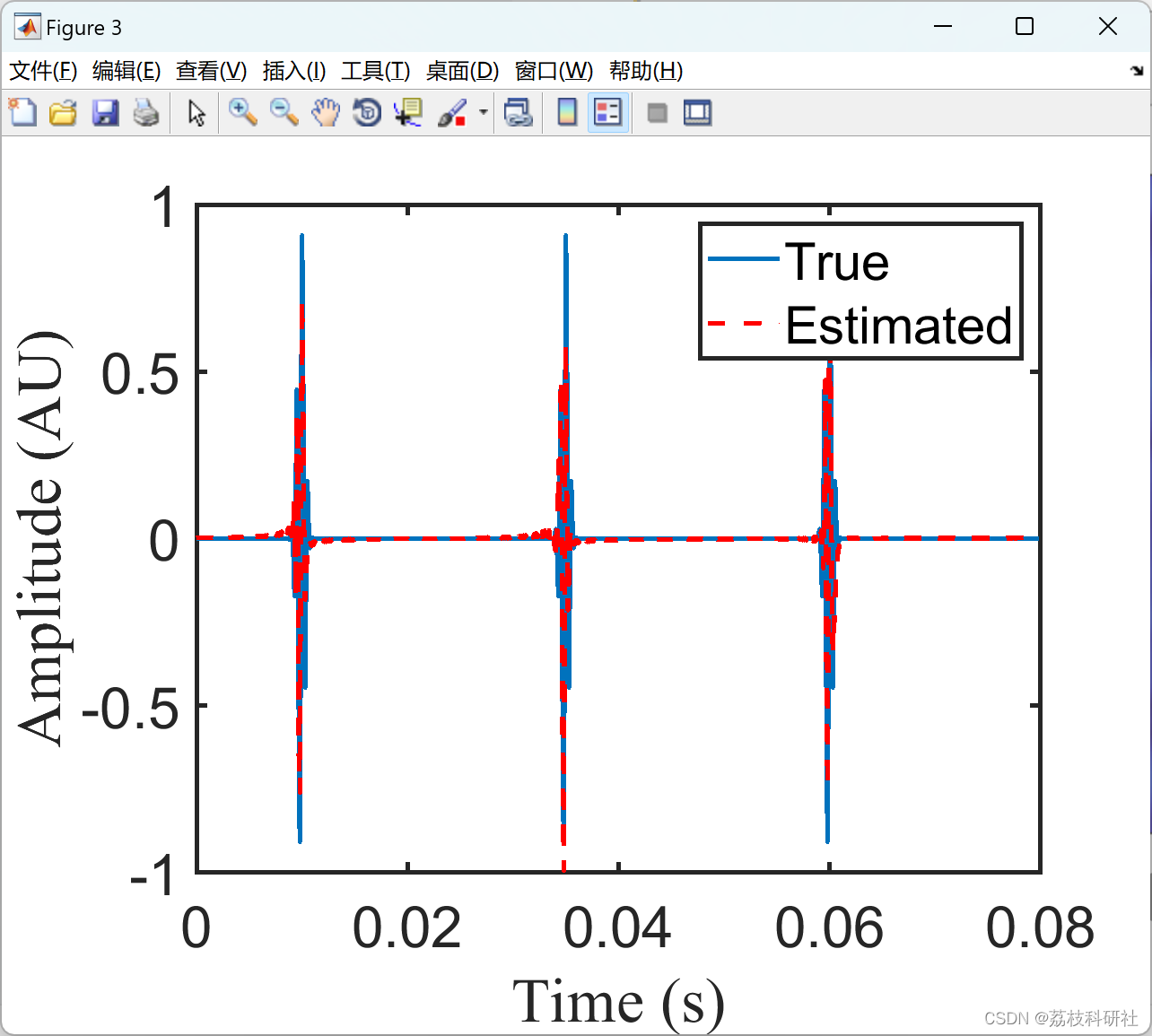
eSig = eM1 + eM2 + eM3; % Reconstructed signal modes

figure
set(gcf,'Position',[20 100 640 500]);        
set(gcf,'Color','w'); 
plot(t,impulse,'linewidth',2);  
hold on
plot(t,eSig,'r--','linewidth',2); 
xlabel('Time (s)','FontSize',24,'FontName','Times New Roman');
ylabel('Amplitude (AU)','FontSize',24,'FontName','Times New Roman');
set(gca,'FontSize',24)
set(gca,'linewidth',2);
legend('True','Estimated')

%%%%% In practice, the above procedure can be executed iteratively until the energy of the residual signal is smaller than a threshold

🎉3 参考文献

部分理论来源于网络，如有侵权请联系删除。

[1]苏理云,石林.卡尔曼滤波下混沌噪声背景中微弱脉冲信号的检测[J].重庆理工大学学报(自然科学),2022,36(09):260-265.

🌈4 Matlab代码实现