
PINN学习与实验(一)
今天第一天接触PINN,用深度学习的方法求解PDE,看来是非常不错的方法。做了一个简单易懂的例子,这个例子非常适合初学者。做了一个小demo, 大家可以参考参考
所用工具
使用了python和pytorch进行实现
python3.6
toch1.10
数学方程
使用一个最简单的常微分方程:
f
′
(
x
)
=
f
(
x
)
(
1
)
f
(
0
)
=
1
(
2
)
f'(x) = f(x) hspace{2cm}(1) \ f(0) = 1 hspace{2.6cm}(2)
f′(x)=f(x)(1)f(0)=1(2)
这个微分方程其实就是:
f
(
x
)
=
e
x
(
3
)
f(x)=e^{x} hspace{2.45cm}(3)
f(x)=ex(3)
模型搭建
核心-使用最简单的全连接层:
class Net(nn.Module):
    def __init__(self, NL, NN): # NL n个l(线性,全连接)隐藏层, NN 输入数据的维数,
        # NL是有多少层隐藏层
        # NN是每层的神经元数量
        super(Net, self).__init__()
        self.input_layer = nn.Linear(1, NN)
        self.hidden_layer = nn.linear(NN,int(NN/2)) ## 原文这里用NN,我这里用的下采样,经过实验验证,“等采样”更优。更多情况有待我实验验证。
        self.output_layer = nn.Linear(int(NN/2), 1)

    def forward(self, x):
        out = torch.tanh(self.input_layer(x))
        out = torch.tanh(self.hidden_layer(out))
        out_final = self.output_layer(out)
        return out_final
偏微分方程定义,也就是公式(1):
def ode_01(x,net):
    y=net(x)
    y_x = autograd.grad(y, x,grad_outputs=torch.ones_like(net(x)),create_graph=True)[0]
    return y-y_x   # y-y' = 0
所有实现代码
一下代码复制粘贴,可直接运行:
import torch
import torch.nn as nn
import numpy as np
import matplotlib.pyplot as plt
from torch import autograd

"""
用神经网络模拟微分方程,f(x)'=f(x),初始条件f(0) = 1
"""

class Net(nn.Module):
    def __init__(self, NL, NN): # NL n个l(线性,全连接)隐藏层, NN 输入数据的维数,
        # NL是有多少层隐藏层
        # NN是每层的神经元数量
        super(Net, self).__init__()
        self.input_layer = nn.Linear(1, NN)
        self.hidden_layer = nn.Linear(NN,int(NN/2)) ## 原文这里用NN,我这里用的下采样,经过实验验证,“等采样”更优。更多情况有待我实验验证。
        self.output_layer = nn.Linear(int(NN/2), 1)

    def forward(self, x):
        out = torch.tanh(self.input_layer(x))
        out = torch.tanh(self.hidden_layer(out))
        out_final = self.output_layer(out)
        return out_final


net=Net(4,20) # 4层 20个
mse_cost_function = torch.nn.MSELoss(reduction='mean') # Mean squared error 均方误差求
optimizer = torch.optim.Adam(net.parameters(),lr=1e-4)  # 优化器

def ode_01(x,net):
    y=net(x)
    y_x = autograd.grad(y, x,grad_outputs=torch.ones_like(net(x)),create_graph=True)[0]
    return y-y_x   # y-y' = 0

# requires_grad=True).unsqueeze(-1)

plt.ion()  # 动态图
iterations=200000
for epoch in range(iterations):

    optimizer.zero_grad()  # 梯度归0

    ## 求边界条件的损失函数
    x_0 = torch.zeros(2000, 1)
    y_0 = net(x_0)
    mse_i = mse_cost_function(y_0, torch.ones(2000, 1))  # f(0) - 1 = 0

    ## 方程的损失函数
    x_in = np.random.uniform(low=0.0, high=2.0, size=(2000, 1))
    pt_x_in = autograd.Variable(torch.from_numpy(x_in).float(), requires_grad=True)  # x 随机数
    pt_y_colection=ode_01(pt_x_in,net)
    pt_all_zeros= autograd.Variable(torch.from_numpy(np.zeros((2000,1))).float(), requires_grad=False)
    mse_f=mse_cost_function(pt_y_colection, pt_all_zeros)  # y-y' = 0

    loss = mse_i + mse_f
    loss.backward()  # 反向传播
    optimizer.step()  # 优化下一步。This is equivalent to : theta_new = theta_old - alpha * derivative of J w.r.t theta

    if epoch%1000==0:
            y = torch.exp(pt_x_in)  # y 真实值
            y_train0 = net(pt_x_in) # y 预测值
            print(epoch, "Traning Loss:", loss.data)
            print(f'times {epoch}  -  loss: {loss.item()} - y_0: {y_0}')
            plt.cla()
            plt.scatter(pt_x_in.detach().numpy(), y.detach().numpy())
            plt.scatter(pt_x_in.detach().numpy(), y_train0.detach().numpy(),c='red')
            plt.pause(0.1)
结果展示
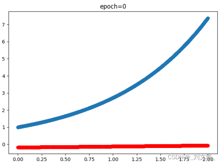
训练0次时的结果也就是没训练,蓝色是真实值、红色是预测值:
训练2000次时的结果,蓝色是真实值、红色是预测值:

训练7000次和13000时的结果,蓝色是真实值、红色是预测值:


训练20000时的结果,蓝色是真实值、红色是预测值,不过红色已经完全把蓝色覆盖了,也就是完全拟合了:

参考文献
[1]. 每天进步一点点吧. PINN学习记录.
https://blog.csdn.net/weixin_45805559/article/details/121574293
相关文章
- EasyCVR对接华为iVS订阅摄像机和用户变更请求接口介绍
- 精选 | 腾讯云CDN内容加速场景有哪些?
- 模块化网络防止基于模型的多任务强化学习中的灾难性干扰
- 用搜索和注意力学习稳健的调度方法
- 用于多变量时间序列异常检测的学习图神经网络
- 助力政企自动化自然生长,华为WeAutomate RPA是怎么做到的?
- 使用腾讯轻量云搭建Fiora聊天室
- TSRC安全测试规范
- 云计算“功守道”
- 助力成本优化,腾讯全场景在离线混部系统Caelus正式开源
- Flink 利器:开源平台 StreamX 简介
- 腾讯云实践 | 一图揭秘腾讯碳中和?解决方案
- 深度学习中的轻量级网络架构总结与代码实现
- 信息系统项目管理师(高项复习笔记三)
- Adobe国际认证让科技赋能时尚
- c++该怎么学习(面试吃土记)
- 面试官问发布订阅模式是在问什么?
- 面试官:请实现一个通用函数把 callback 转成 promise
- 空中悬停、翻滚转身、成功着陆,我用强化学习「回收」了SpaceX的火箭
- 中山大学林倞解读视觉语义理解新趋势:从表达学习到知识及因果融合