
Tree - Information Theory
This will be a series of post about Tree model and relevant ensemble method, including but not limited to Random Forest, AdaBoost, Gradient Boosting and xgboost.
So I will start with some basic of Information Theory, which is an importance piece in Tree Model. For relevant topic I highly recommend the tutorial slide from Andrew moore
What is information?
Andrew use communication system to explain information. If we want to transmit a series of 4 characters ( ABCDADCB... ) using binary code ( 0&1 ). How many bits do we need to encode the above character?
The take away here is the more bit you need, the more information it contains.
I think the first encoding coming to your mind will be following:
A = 00, B=01, C =10, D=11. So on average 2 bits needed for each character.
Can we use less bit on average?
Yes! As long as these 4 characters are not uniformally distributed.
Really? Let's formulate the problem using expectation.
where P( x=k ) is the probability of character k in the whole series, and n_k is the number of bits needed to encode k. For example: P( x=A ) = 1/2, P( x=B ) = 1/4, P( x=c ) = 1/8, P( x=D ) = 1/8, can be encoded in following way: A=0, B=01, C=110, D=111.
Basically we can take advantage of the probability and assign shorter encoding to higher probability variable. And now our average bit is 1.75 < 2 !
Do you find any other pattern here?
the number of bits needed for each character is related to itsprobability : bits = -log( p )
Here log has 2 as base, due to binary encoding
We can understand this from 2 angles:
- How many value can n bits represent? \(2^n\), where each value has probability \(1/2^n\), leading to n = log(1/p).
- Transmiting 2 characters independently: P( x1=A, x2 =B ) = P( x1=A ) * P( x2=B ), N( x1, x2 ) = N( x1 ) + N( x2 ), where N(x) is the number of bits. So we can see that probability and information is linked via log.
In summary, let's use H( X ) to represent information of X, which is also known as Entropy
when X is discrete, \(H(X) = -\sum_i{p_i \cdot log_2{p_i}}\)
when X is continuous, \(H(X) = -\int_x{p(x) \cdot log_2{p(x)}} dx\)
Deeper Dive into Entropy
1. Intuition of Entropy
I like the way Bishop describe Entropy in the book Pattern Recognition and Machine Learning. Entropy is 'How big the surprise is'. In the following post- tree model, people prefer to use 'impurity'.
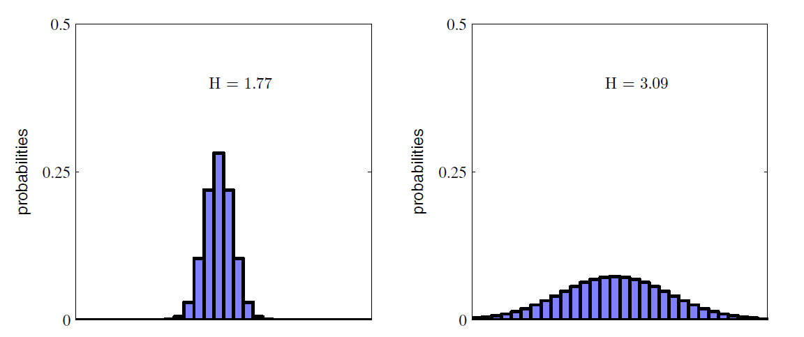
Therefore if X is a random variable, then the more spread out X is, the higher Entropy X has. See following:
2. Conditional Entropy
Like the way we learn probability, after learning how to calculate probability and joint probability, we come to conditional probability. Let's discuss conditional Entropy.
H( Y | X ) is given X, how surprising Y is now? If X and Y are independent then H( Y | X ) = H( Y ) (no reduce in surprising). From the relationship between probability and Entropy, we can get following:
Above equation can also be proved by entropy. Give it a try! Here let's go through an example from Andrew's tutorial to see what is conditional entropy exactly.
X = college Major, Y = Like 'Gladiator'
| X | Y |
|---|---|
| Math | YES |
| History | NO |
| CS | YES |
| Math | NO |
| Math | NO |
| CS | YES |
| History | NO |
| Math | YES |
Let's compute Entropy using above formula:
H( Y ) = -0.5 * log(0.5) - 0.5 * log(0.5) = 1
H( X ) = -0.5 * log(0.5) - 0.25 * log(0.25) - 0.25 * log(0.25) = 1.5
H( Y | X=Math ) = 1
H( Y | X=CS ) = 0
H( Y | X=History ) = 0
H( Y | X ) = H( Y | X=Math ) * P( X=Math ) + H( Y | X=History ) * P( X=History ) + H( Y | X =CS ) * P( X=CS ) = 0.5
Here we see H( Y | X ) < H( Y ), meaning knowing X helps us know more about Y.
When X is continuous, conditional entropy can be deducted in following way:
we draw ( x , y ) from joint distribution P( x , y ). Given x, the additional information on y becomes -log( P( y | x ) ). Then using entropy formula we get:
In summary
When X is discrete, \(H(Y|X) = \sum_j{ H(Y|x=v_j) p(x=v_j)}\)
When X is continuous, \(H(Y|X) = \int_x{ H(Y|x)p(x) dx}\)
3. Information Gain
If we follow above logic, then information Gain is the reduction of surpise in Y given X. So can you guess how IG is defined now?
IG = H( Y ) - H( Y | X )
In our above example IG = 0.5. And Information Gain will be frequently used in the following topic - Tree Model. Because each tree splitting aims at lowering the 'surprising' in Y, where the ideal case is that in each leaf Y is constant. Therefore split with higher information is preferred
So far most of the stuff needed for the Tree Model is covered. If you are still with me, let's talk a about a few other interesting topics related to information theory.
Other Interesting topics
Maximum Entropy
It is easy to know that when Y is constant, we have the smallest entropy, where H( Y ) = 0. No surprise at all!
Then how can we achieve biggest entropy. When Y is discrete, the best guess will be uniform distribution. Knowing nothing about Y brings the biggest surprise. Can we prove this ?
All we need to do is solving a optimization with Lagrange multiplier as following:
Where we can solve hat p are equal for each value, leading to a uniform distribution.
What about Y is continuous? It is still an optimization problem like following:
We will get Gaussian distribution! You want to give it a try?!
Relative Entropy
Do you still recall our character transmitting example at the very beginning? That we can take advantage of the distribution to use less bit to transmit same amount of information. What if the distribution we use is not exactly the real distribution? Then extra bits will be needed to send same amount of character.
If the real distribution is p(x) and the distribution we use for encoding character is q(x), how many additional bits will be needed? Using what we learned before, we will get following
Does this looks familiar to you? This is also know as Kullback-Leibler divergence, which is used to measure the difference between 2 distribution.
And a few features can be easily understood in terms of information theory:
- KL( p || q ) >= 0, unless p = q, additional bits are always needed.
- KL( p || q) != KL( q || p ), because data originally follows 2 different distribution.
To be continued.
reference
- Andrew Moore Tutorial http://www.cs.cmu.edu/~./awm/tutorials/dtree.html
- Bishop, Pattern Recognition and Machine Learning 2006
- T. Hastie, R. Tibshirani and J. Friedman. “Elements of Statistical Learning”, Springer, 2009.
相关文章
- 在 Go 里用 CGO?这 7 个问题你要关注!
- 9款优秀的去中心化通讯软件 Matrix 的客户端
- 求职数据分析,项目经验该怎么写
- 在OKR中,我看到了数据驱动业务的未来
- 火山引擎云原生大数据在金融行业的实践
- OpenHarmony富设备移植指南(二)—从postmarketOS获取移植资源
- 《数据成熟度指数》报告:64%的企业领袖认为大多数员工“不懂数据”
- OpenHarmony 小型系统兼容性测试指南
- 肯睿中国(Cloudera):2023年企业数字战略三大趋势预测
- 适用于 Linux 的十大命令行游戏
- GNOME 截图工具的新旧截图方式
- System76 即将推出的 COSMIC 桌面正在酝酿大变化
- 2GB 内存 8GB 存储即可流畅运行,Windows 11 极致精简版系统 Tiny11 发布
- 迎接 ecode:一个即将推出的具有全新图形用户界面框架的现代、轻量级代码编辑器
- loongarch架构介绍(三)—地址翻译
- Go 语言怎么解决编译器错误“err is shadowed during return”?
- 敏捷:可能被开发人员遗忘的部分
- Denodo预测2023年数据管理和分析的未来
- 利用数据推动可持续发展
- 在 Vue3 中实现 React 原生 Hooks(useState、useEffect),深入理解 React Hooks 的